Copyright © 2011-2014 airxc.com, airxcell.com
Table of Contents
This dynamic form is about portfolio optimization from the perspective of computational finance and financial engineering. Thus the main emphasis here is to briefly introduce the concepts and to give the user a set of powerful tools to solve the problems in the field of portfolio optimization. It provides a way to optimize a portfolio of assets. The goal is to determine the asset weights that minimize the risk for a desired return or, alternatively, that maximize the return for a given risk.
After determining the optimal weights it is advisable to conduct a performance analysis on the optimal portfolio. However, before you can optimize a portfolio, you have to create an environment which specifies a portfolio from the beginning and defines all the parameters and values that are required to perform the optimization. In the provided form, one describes the portfolio environment including the specification of all parameters describing the portfolio, the selection and description of the assets data set for which we want to optimize the portfolio, and to set the constraints under which the portfolio will be optimized.
Any timeseries already loaded by the user within the R environment (using commands or whatever) compliant with a
xts, zoo or timeSeries timeseries can be used
as a constituent. Moreover, the user can use the
Manage assets (10)
dynamic form to load constituents which is the preferred way since it loads additional data such as
the name of the asset, its currency, etc.
A new "6. Portfolio Optimization" form can be added to the workspace by using
Form → 6. Portfolio Optimization
(![]() )
)
The theory behind the portfolio optimization algorithms available within this dynamic form is presented in the chapter Chapter 17, Portfolio Optimization theory.
The portfolio optimization procedure works with returns instead of asset values. The whole optimization procedure is most often used to optimize (thus maximize) returns. In other cases it is intended to optimize (thus minimize) risk (hence volatility, i.e. the variance of returns). Section 17.1.1, “Asset returns” discusses how asset returns are computed.
The portfolio score function (i.e. the value to be optimized) is most often a question of minimizing the risk (the variance, covariance, whatever...) or maximizing the portfolio return. Section 17.1.2, “Portfolio return” discusses how the portfolio return is computed from asset returns.
The Portfolio (15) dynamic form uses several functions and methods provided by Rmetrics to compute basic statistics of financial time series from S4 timeSeries objects. These include summary and basic statistics, drawdown statistics, sample mean and covariance estimation, quantile and risk estimation, amongst others. Moreover, there are functions to compute column statistics and cumulated column statistics, which are very important tools used by the portfolio optimization procedure.
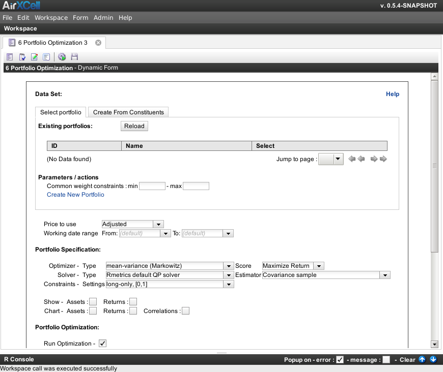
A newly created "6. Portfolio Optimization" dynamic form looks as shown on Figure 15.1, “New '6. Portfolio Optimization' dynamic form”.
In AirXCell and R financial packages in general, data sets are represented by S4 timeSeries objects. These objects are used to represent financial data for portfolio optimization. Returns for a price or index series are computed by the Portfolio (15) dynamic form when optimizing portfolio from the selected assets.
This first section of the screen shows the loaded assets available as portfolio constituents. Constituents can be selected one at a time using the checkbox on the right-most column of the constituents list or all together using the buttons on the bottom of the list.
In addition to viewing and selecting constituents, the list enables the user to specify a minimum weight in percentage and a maximum weight for each constituent. This is the most simple form of constraints that can be specified on the target portfolio.
The loaded assets from the quantmod - Manage Assets (10) form usually provide five different quotes : daily Open and Close, daily High and Low and Adjustedprice.
The user can choose what price she wants to use to compute the returns. The price to use is chosen globally, i.e. the same one is used for every asset.
As described below for Mean-Variance (Markovitz) and Mean-conditional value at risk portfolios, the optimization algorithms work with mean, variance or covariance, etc. values computed from the asset returns.
By default, the timeseries considered for computing these values are taken into account starting with the latest start date of every asset timeseries and ending with the earliest end date. The user can however choose a subset of that default period by specifying here different dates.
To compose and optimize a portfolio of assets we first have to specify it. This process includes choosing the kind of portfolio model we want to investigate, choosing the required portfolio parameter settings, and choosing which type of programming solver (linear, quadratic, nonlinear) should be applied.
The user can choose amongst every supported currency as the portfolio currency. A portfolio is inevitably computed in a specific currency, the default is USD (US Dollar). Assets can be loaded in any currency. Whenever the portfolio contains an asset loaded in a different currency that the portfolio currency, it is first converted in the target portfolio currency before being taken into account for the returns calculation. Any FOREX (See Chapter 11, Form : 2. Manage FOREX) required for such a conversion is loaded automatically and transparently.
-
Mean-Variance (Markowitz) : Modern portfolio theory[5] proposes how rational investors use diversification to optimize their portfolio(s) of risky assets. The basic concepts of the theory go back to Markowitz’s idea of diversification and the efficient portfolio frontier. His model considers asset returns as a random variable, and models a portfolio as a weighted combination of assets. Being a random variable, a portfolio’s returns have an expected mean and variance. In this model, return and risk are estimated by the sample mean and the sample standard deviation of the asset returns.
The problem of minimizing the covariance risk for a given target return with optional box and group constraints is a quadratic programming problem with linear constraints. The opposite case, fixing the risk and maximizing the return, has a linear objective function with quadratic constraints. This second problem is much more complex than the first one. If we have even more complex constraints, i.e. nonlinear constraints, we need a new class of solvers called non-linear constrained portfolio problem. This allows us to handle the case of linear and quadratic objective functions with non-linear constraints. In all three cases we speak of Markowitz’ portfolio optimization problem, although they require different classes of solvers with increasing complexity.
The theory behind the optimization algorithm for Markowitz' Mean-Variance portfolio is presented in details in the next chapter Chapter 17, Portfolio Optimization theory in section Markowitz Portfolio Theory.
-
Mean-conditional value at risk : An alternative risk measure to the covariance is the Conditional Value at Risk, CVaR, which is also known as mean excess loss, mean shortfall or tail Value at Risk, VaR. For a given time horizon and confidence level, CVaR is the conditional expectation of the loss above VaR for the time horizon and the confidence level under consideration.
In the mean-CVaR portfolio model, covariance risk is now replaced by the conditional Value at Risk [1] [4] as the risk measure. In contrast to the mean-variance portfolio optimization problem, we no longer restrict the set of assets to have a multivariate elliptically contoured distribution.
The theory behind the optimization algorithm for Mean-conditional value at risk portfolios is presented in details in the Chapter 17, Portfolio Optimization theory, Mean-CVaR Portfolio Theory.
The two available options are either minimizing the portfolio’s risk for a given target return or maximizing the portfolio’s return for a given target risk. In the default case of the meanvariance portfolio, the target risk is calculated from the sample covariance (or an alternative measure, e.g. a robust covariance estimate). The target return is computed by the sample mean of the assets if not otherwise specified.
The optimization procedure needs to start with a feasible solution. In addition, it can only optimize one single score function at a time[10]. This means that it can either optimite returns or risks, not both at a time. There is however a trick to optimize both at a time which consists in using the return / risk ratio as the score function.
The single score functions limitation implies that the optimizier requires a predefined target acceptable risk when maximizing the return or a predefined target return when minimizing risks.
In the current version of the Portfolio dynamic form, the user has two choices to specifiy the predefined acceptable risk (in the case of a return maximization) or the predefined target return (in the case of a risk minimization):
-
The default choice for both these settings is to use the values computed from the Feasible portfolio (15.5.2). This is an easy go since the user does not need to worry about these values but it might be uneffective since the values from the feasible portfolio (initial solution) might well be suboptimal.
The user can also uncheck the usage of the default values and input its own values. Giving feasible specific values can well be very tricky so the best approach here is to do a first run by using the default values, see what values have been used and then from here guess the values that might be more optimal and input them here.
The name of the default solver used for the optimization of the mean-variance Markowitz portfolio, which is the default portfolio, is a quadratic programming (QP) solver. This solver implements the approach of QP Goldfarb and Idnani[9].
For mean-CVaR portfolio optimization, one should use a linear programming (LP) solver. This solver uses R’s interface to the GNU linear programing kit (GLPK).
It is very important to be careful when modifying specification settings, because there are settings that are incompatible with others. For example, if you want to minimize the covariance risk for a mean-variance portfolio, you cannot assign a linear programming solver.
Currently we are working on implementing more consistency checks for the specification settings, so that the user wont have to worry about creating conflicting settings. However, this has not been fully implemented in the current version of the Portfolio dynamic form.
-
Minimum covariance determinant : This method estimates a robust mean and covariance by the minimum covariance determinant estimator. The Minimum Covariance Determinant method consists in searching for the half of the data that is most tightly clustered together amongst all subsets containig half of the data, as measured by the generalized variance. Recall that for the determinant of the variance (the generalized variance) to be relatively small, it must be the case that there are no outliers.
-
Minimum volume ellipsoid : This method is used for robust outlier detection in multivariate space. The algorithm takes subsamples of the dataset and calculates the Volume of the Ellipsoid representing that subsample. Outliers increase the volume dramatically, so the Minimum Volume Ellipsoid (MVE) will correspond with the actual core of the dataset. After this, data points exceeding the cut-off value for the Mahalanobis distance will be designated outliers and are discarded. The MVE is implemented in R's recommended package MASS.
-
Orthogonalized Gnanadesikan-Kettenring : The "OGK" method computes the orthogonalized pairwise covariance matrix estimate described in Maronna & Zamar (2002). The estimator is implemented in the contributed R package robustbase .
-
Shrinkage : The "shrink" method provides robust covariance estimation by the shrinkage method [12]. The shrinkage function is implemented in the contributed R package corpcor.
-
Bagged : The "bagged" method provides a variance-reduced estimator of the covariance matrix using bootstrap aggregation, hence the name "bagged"[13]. "bagged" was implemented in a previous version of the contributed R package corpcor.
Constraints define restrictions and boundary conditions on the weights and functional measures, depending on, or derived from, the portfolio weights. Constraints are defined by a character string or a vector of character strings. The formal style of these strings can be used like a language to express lower and upper bounds on the ranges of weights that have to be satisfied for box, group, covariance risk budgets and general non-linear constraint settings.
In order to simplify the process, however, two specific cases of constraints definition are supported by the system out of the box, i.e. without the user requiring the hassle of defining manually the constraints using the constraint language. These are the following :
Short : short constraints, sets lower and upper bounds of weights as box constraints ranging between minus and plus infinity for all assets. The setting allows for unlimited negative and positive weights. In this case, the mean-variance portfolio optimization problem can be solved analytically.
Long Only : long-only constraints, sets lower and upper bounds of weights as box constraints. Long-only positions reflect the fact that all weights are allowed to be between zero and one. Do not confuse this setting with box constraints, where the weights are restricted by arbitrary negative and/or positive lower and upper bounds.
We introduce here the rules to express constraints as strings and introduce the functions used to create a summary for all the constraints.
-
LongOnly: long-only constraints [0,1] -
Short: unlimited short selling, [-Inf,Inf] -
minW[<...>]=<...>: lower box bounds = lower bounds of weights for box constraintsExample :
minW[1:3] = 0.1 -
maxw[<...>]=<...>: upper box bounds = upper bounds of weights for box constraintsExample :
maxW[c(1, 3)] = c(0.5, 0.6) -
eqsumW[<...>]=<...>: equality group constraintsExample :
eqsumW[c(\"SPI\", \"SII\")]=0.6 -
minsumW[<...>]=<...>: lower group boundsExample :
minsumW[c(2, 3)]=0.2 -
maxsumW[<...>]=<...>: upper group boundsExample :
maxsumW[1:nAssets]=0.7 -
minB[<...>]=<...>: lower covariance risk budget boundsExample :
minB[1:nAssets]=-Inf -
maxB[<...>]=<...>: upper covariance risk budget boundsExample :
maxB[c(1, 2:nAssets)]=c(0.5, rep(0.6, times=2)) -
listF=list(<...>): list of non-linear functions -
minf[<...>]=<...>: lower bounds of non-linear functions -
maxf[<...>]=<...>: upper bounds of non-linear functions
When selected, this causes the execution of the form to end up with Data Frame module instances to be created and added to the workspace in order to display either the assets composing the portfolio themselves or the returns computed from the assets.
After we have set the data, specified the portfolio settings, and defined the constraints, we are ready to optimize the portfolio. The portfolio optimization functions take the data, the specifications and the constraints as inputs.
Here, the user can choose whether he wants to run the optimization algorithm or not. Running the optimization algorithm is a prerequisite to the features available below such as Portfolio Analysis . It is however possible to disable the optimization procedure. This is useful for instance when the user is in a constituent selection phase and simply wants to display or charts the assets or the returns without running the optimizer yet.
The portfolio optimization procedure needs to start with a feasible solution, i.e. an initial portfolio. In our case, the single feasible solution currently supported by the Portfolio (15) dynamic form is an Equally weighted portfolio, i.e. a portfolio where each and every consituent has a equals weight. This situation is kind of like a portfolio where any analyst bough the same volume of security, for instance 1k USD of IBM, 1k USD of Microsoft, and so on.
The initial weights of the feasible portfolio can be chartted using the related checkbox. The result is shown on Figure 15.2, “Equally weighting portfolio example”.
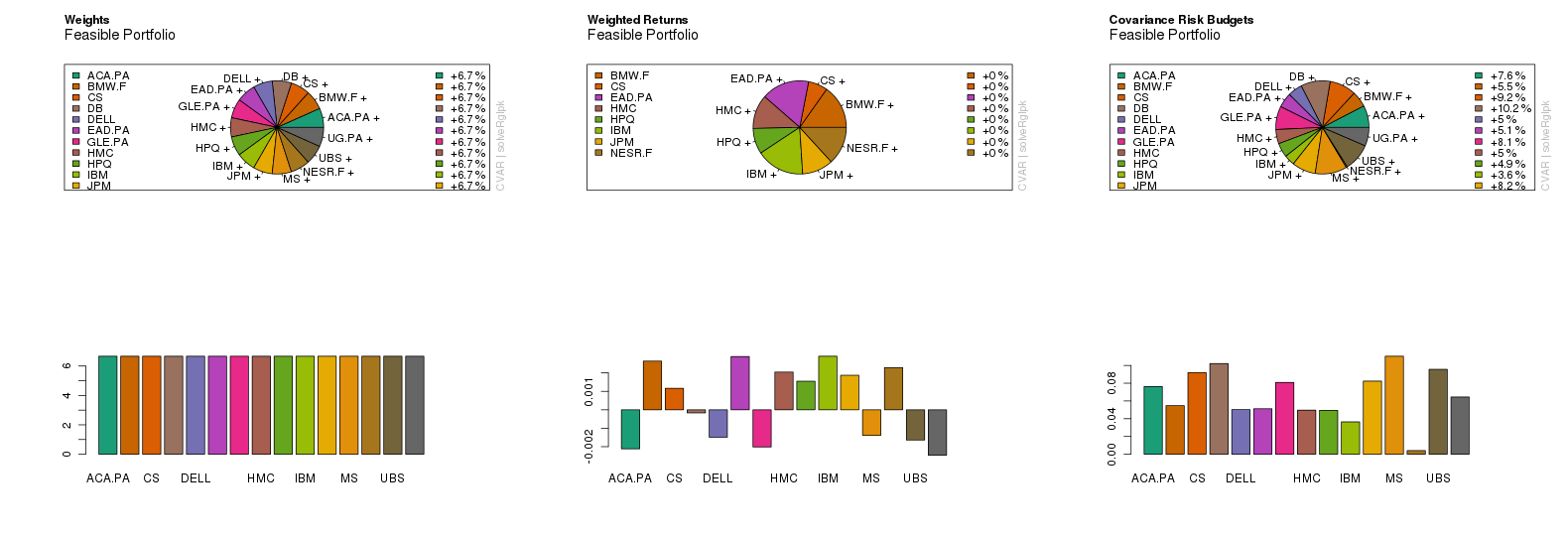
In adition, in the textual results window, the feasible portfolio is displayed:
 --------------------------------------------------------------------------------

 INITIAL FEASIBLE SOLUTION
 -------------------------

 Feasible portfolio:


 Title:
  CVAR Feasible Portfolio
  Estimator:         covEstimator
  Solver:            solveRglpk
  Optimize:          minRisk
  Constraints:       LongOnly

 Portfolio Weights:
   AAPL    ABB     CS    HMC    HPQ    IBM     MS     SI    SNE    UBS   YHOO
 0.0909 0.0909 0.0909 0.0909 0.0909 0.0909 0.0909 0.0909 0.0909 0.0909 0.0909

 Covariance Risk Budgets:
   AAPL    ABB     CS    HMC    HPQ    IBM     MS     SI    SNE    UBS   YHOO
 0.0722 0.1031 0.1089 0.0635 0.0715 0.0519 0.1297 0.0947 0.0725 0.1441 0.0878

 Target Return and Risks:
   mean     mu    Cov  Sigma   CVaR    VaR
 0.0001 0.0001 0.0195 0.0195 0.0471 0.0293

 Description:
  Tue Jun 26 10:08:03 2012 by user:
Markowitz' Modern portfolio theory states that an investor may choose to exchange risk for return along a curve known as the Efficient frontier. Since it is inefficient to incur a given level of risk when one can rearrange the portfolio to achieve a greater expected return for the same risk, there is a strong motivation to optimize.
The Portfolio Optimization algorithm calculates the optimal capital weightings for a set of assets that gives the highest return for the least risk, or the lowest risk for a target return. The ability to apply optimization analysis to a portfolio of assets represents an excellent framework for driving capital allocation, investment, and divestment decisions.
-
Efficient : Maximize returns or minimize risks according to the setting given on the portfolio specification.
When maximizing returns, the optimizer currently only assumes a target accpetable risk value as computed for the initial feasible portfolio (equally weighted).
When minimizing the risk, the optimizer currently only assumes a target return value as computed for the initial feasible portfolio (equally weighted).
-
Maximum possible ratio return/risk at all : computes the portfolio with the highest return/risk ratio
-
Minimum possible risk at all : computes the portfolio with the lowest risk at all
The resulting weights of the optimized portfolio can be chartted using the related checkbox. The result is shown on Figure 15.3, “Optimized portfolio example”.
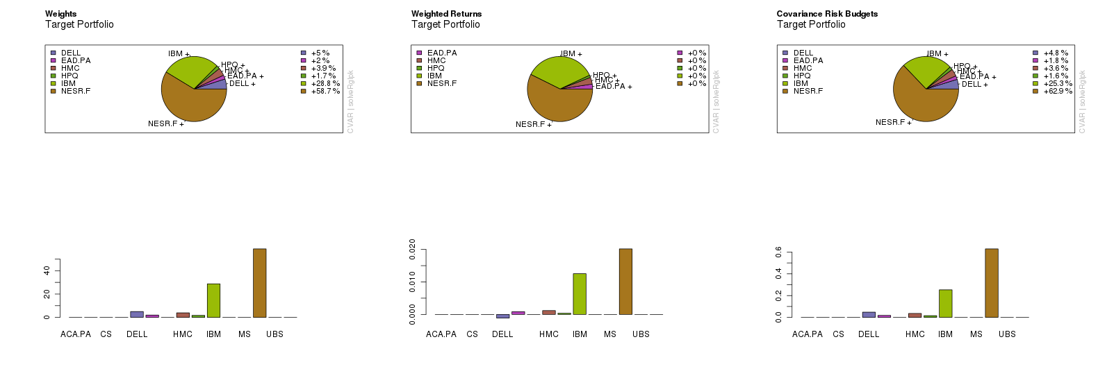
In adition, in the textual results window, the target optimized portfolio is displayed:
 --------------------------------------------------------------------------------

 OPTIMIZED SOLUTION
 ------------------

 Target portfolio specs:
 -----------------------


 Model List:
  Type:                      CVAR
  Optimize:                  minRisk
  Estimator:                 covEstimator
  Tail Risk:                 list()
  Params:                    alpha = 0.05 a = 1

 Portfolio List:
  Portfolio Weights:         NA
  Target Return:             1e-04
  Target Risk:               NA
  Risk-Free Rate:            0
  Number of Frontier Points: 50
  Status:                    NA

 Optim List:
  Solver:                    solveRglpk
  Objective:                 list()
  Options:                   meq = 2
  Control:                   list()
  Trace:                     FALSE

 Message List:
  List:                      NULL

 Target portfolio:
 -----------------


 Title:
  CVAR Efficient Portfolio
  Estimator:         covEstimator
  Solver:            solveRglpk
  Optimize:          minRisk
  Constraints:       LongOnly

 Portfolio Weights:
   AAPL    ABB     CS    HMC    HPQ    IBM     MS     SI    SNE    UBS   YHOO
 0.0000 0.0000 0.0000 0.1474 0.0635 0.5649 0.0000 0.0000 0.2242 0.0000 0.0000

 Covariance Risk Budgets:
   AAPL    ABB     CS    HMC    HPQ    IBM     MS     SI    SNE    UBS   YHOO
 0.0000 0.0000 0.0000 0.1407 0.0627 0.5308 0.0000 0.0000 0.2658 0.0000 0.0000

 Target Return and Risks:
   mean     mu    Cov  Sigma   CVaR    VaR
 0.0001 0.0001 0.0151 0.0151 0.0357 0.0241

 Description:
  Tue Jun 26 10:08:05 2012 by user:
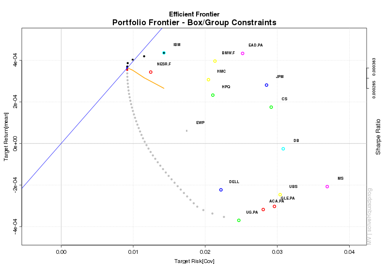
The efficient frontier together with the minimum variance locus form the upper border and lower border lines of the feasible set. To the right the feasible set is determined by the envelope of all pairwise asset frontiers. The region outside of the feasible set is unachievable by holding risky assets alone. No portfolios can be constructed corresponding to the points in this region. Points below the frontier are suboptimal. Thus, a rational investor will hold a portfolio only on the frontier.
The portfolio frontier feature on the Portfolio (15) dynamic form computes the whole efficient frontier of a portfolio and shows the result in a graphical way. For the default settings with long-only constraints, the range spans all values equidistantly ranging from the asset with the lowest return up to the asset with the highest return. Allowing for box, group and other more complex constraints the range of the frontier will be downsized, i.e. the length of the frontier becomes shorter and shorter. Bear in mind that it is possible for the constraints to be too strong, and that a frontier might not even exist at all.
Number of Frontier Points : the number of points to be tried when seaking for the frontier.
The resulting efficient frontier can be chartted using the related checkbox. The result is shown on figure Figure 15.4, “Efficient frontier example”.
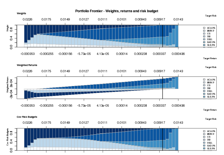
In adition, in the textual results window, the efficient frontier is displayed:
 --------------------------------------------------------------------------------

 PORTFOLIO FRONTIER
 ------------------

 Portfolio Frontier:


 Title:
  MV Portfolio Frontier
  Estimator:         covEstimator
  Solver:            solveRquadprog
  Optimize:          minRisk
  Constraints:       LongOnly
  Portfolio Points:  5 of 49

 Portfolio Weights:
      AAPL    ABB     CS    HMC    HPQ    IBM     MS     SI    SNE    UBS   YHOO
 1  0.0000 0.0000 0.0000 0.0000 0.0713 0.0000 0.0000 0.0000 0.9089 0.0198 0.0000
 13 0.0000 0.0000 0.0000 0.1056 0.1091 0.4858 0.0000 0.0000 0.2996 0.0000 0.0000
 25 0.1852 0.0000 0.0000 0.2272 0.0000 0.5876 0.0000 0.0000 0.0000 0.0000 0.0000
 37 0.5907 0.0000 0.0000 0.0868 0.0000 0.3226 0.0000 0.0000 0.0000 0.0000 0.0000
 49 1.0000 0.0000 0.0000 0.0000 0.0000 0.0000 0.0000 0.0000 0.0000 0.0000 0.0000

 Covariance Risk Budgets:
      AAPL    ABB     CS    HMC    HPQ    IBM     MS     SI    SNE    UBS   YHOO
 1  0.0000 0.0000 0.0000 0.0000 0.0365 0.0000 0.0000 0.0000 0.9489 0.0146 0.0000
 13 0.0000 0.0000 0.0000 0.0959 0.1109 0.4236 0.0000 0.0000 0.3696 0.0000 0.0000
 25 0.2270 0.0000 0.0000 0.2123 0.0000 0.5606 0.0000 0.0000 0.0000 0.0000 0.0000
 37 0.7694 0.0000 0.0000 0.0453 0.0000 0.1853 0.0000 0.0000 0.0000 0.0000 0.0000
 49 1.0000 0.0000 0.0000 0.0000 0.0000 0.0000 0.0000 0.0000 0.0000 0.0000 0.0000

 Target Return and Risks:
       mean      mu     Cov   Sigma    CVaR     VaR
 1  -0.0005 -0.0005  0.0221  0.0221  0.0516  0.0339
 13  0.0000  0.0000  0.0155  0.0155  0.0365  0.0248
 25  0.0005  0.0005  0.0151  0.0151  0.0357  0.0235
 37  0.0010  0.0010  0.0190  0.0190  0.0427  0.0294
 49  0.0015  0.0015  0.0258  0.0258  0.0567  0.0395

 Description:
  Fri Jun 29 12:55:12 2012 by user:
 bench ~ AAPL + ABB + CS + HMC + HPQ + IBM + MS + SI + SNE + UBS +
     YHOO
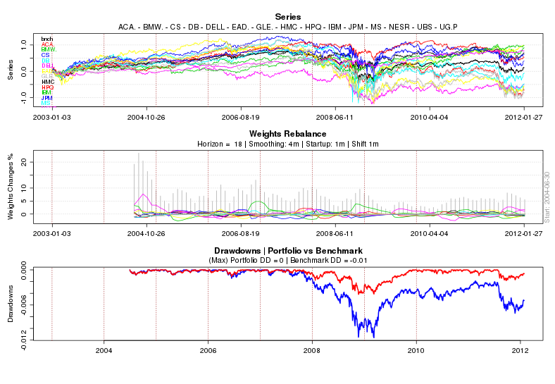
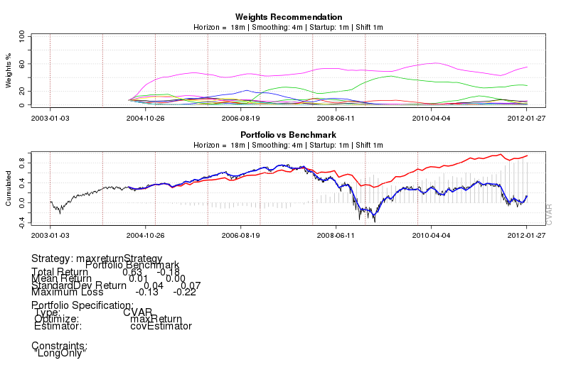
Backtesting is a key component of portfolio management and it is often used to assess and compare different statistical models. Portfolio backtesting is accomplished by reconstructing, with historical data, trades that would have occurred in the past using rules defined by a given strategy. The underlying theory is that any strategy that worked well in the past is likely to work well in the future.
The backtesting results offer statistics that can be used to gauge the effectiveness of the strategy. However, the results achieved from the backtest are highly dependent on the movements of the tested period. Therefore, it is often a good idea to backtest over a long time frame that encompasses several different types of market conditions.
Window Horizon (in months) : The number of months to be taken into accoun in the past to compute the mean (returns), variance and covariance. At each rebalancing point in time, only that amount of data in the past are taken into consideration in the calculations.
Number of months smothing : The number of months to be taken into accoun by the Exponential Moving Average (EMA) smoother. The intent in smoothing is to avoid too many changes in weights each month (avoid to many buy / sell orders).
The resulting backtest can be chartted using the related checkbox. The result is shown on Figure 15.5, “Portfolio backtesting example”.
In adition, in the textual results window, the backtesting is displayed:
 --------------------------------------------------------------------------------

 PORTFOLIO BACKTESTING
 ---------------------

 Portfolio Back-test - specs:


 Model List:
  Type:                      CVAR
  Optimize:                  maxReturn
  Estimator:                 covEstimator
  Tail Risk:                 list()
  Params:                    alpha = 0.05 a = 1

 Portfolio List:
  Portfolio Weights:         NA
  Target Return:             NA
  Target Risk:               0.02925016
  Risk-Free Rate:            0
  Number of Frontier Points: 50
  Status:                    NA

 Optim List:
  Solver:                    solveRglpk
  Objective:                 list()
  Options:                   meq = 2
  Control:                   list()
  Trace:                     FALSE

 Message List:
  List:                      NULL

 Portfolio Back-test - constraints:

 "LongOnly"            "maxW[\\"AAPL\\"] = NA" "minW[\\"AAPL\\"] = NA"
 "maxW[\\"ABB\\"] = NA"  "minW[\\"ABB\\"] = NA"  "maxW[\\"CS\\"] = NA"
 "minW[\\"CS\\"] = NA"   "maxW[\\"HMC\\"] = NA"  "minW[\\"HMC\\"] = NA"
 "maxW[\\"HPQ\\"] = NA"  "minW[\\"HPQ\\"] = NA"  "maxW[\\"IBM\\"] = NA"
 "minW[\\"IBM\\"] = NA"  "maxW[\\"MS\\"] = NA"   "minW[\\"MS\\"] = NA"
 "maxW[\\"SI\\"] = NA"   "minW[\\"SI\\"] = NA"   "maxW[\\"SNE\\"] = NA"
 "minW[\\"SNE\\"] = NA"  "maxW[\\"UBS\\"] = NA"  "minW[\\"UBS\\"] = NA"
 "maxW[\\"YHOO\\"] = NA" "minW[\\"YHOO\\"] = NA"

 Portfolio Back-test - specifications:


 Backtest Specification:

  Windows Function:            equidistWindows
  Windows Params:
   - horizon                   18m

  Strategy Function:           maxreturnStrategy
  Strategy Params:

  Smoother Function:           emaSmoother
  Smoother Params:
   - doubleSmoothing           TRUE
   - lambda                    4m
   - skip                      0
   - initialWeights            0.090 0.090 0.090 0.090 0.090 0.090 0.090 0.090 0.090 0.090 0.090

  Messages:


 Portfolio Back-test - benchmark name:

 "bench"

 Portfolio Back-test - asset names:

 "AAPL" "ABB"  "CS"   "HMC"  "HPQ"  "IBM"  "MS"   "SI"   "SNE"  "UBS"
 "YHOO"

 Portfolio Back-test - weights head :

                  AAPL        ABB         CS       HMC        HPQ       IBM
 2002-09-30 0.02296009 0.02332558 0.02535847 0.2467281 0.06571699 0.2824776
 2002-10-31 0.02466763 0.01220238 0.02837879 0.2577551 0.09897073 0.2995721
 2002-11-30 0.01961186 0.00000000 0.00000000 0.2251096 0.00000000 0.2471409
 2002-12-31 0.01961186 0.00000000 0.00000000 0.2251096 0.00000000 0.2471409
 2003-01-31 0.03455937 0.00000000 0.00000000 0.2147919 0.00000000 0.2475617
 2003-02-28 0.03455937 0.00000000 0.00000000 0.2147919 0.00000000 0.2475617
                   MS         SI       SNE        UBS YHOO
 2002-09-30 0.0147636 0.03338133 0.2600091 0.02527917    0
 2002-10-31 0.0000000 0.04144408 0.2095620 0.02744724    0
 2002-11-30 0.0000000 0.00000000 0.2569992 0.25113849    0
 2002-12-31 0.0000000 0.00000000 0.2569992 0.25113849    0
 2003-01-31 0.0000000 0.00000000 0.2590124 0.24407464    0
 2003-02-28 0.0000000 0.00000000 0.2590124 0.24407464    0

 Portfolio Back-test - weights tail :

                 AAPL ABB CS        HMC HPQ       IBM MS SI SNE UBS       YHOO
 2011-11-30 0.2920445   0  0 0.02565682   0 0.5999402  0  0   0   0 0.08235847
 2011-12-31 0.2944144   0  0 0.06190774   0 0.5396281  0  0   0   0 0.10404975
 2012-01-31 0.2944144   0  0 0.06190774   0 0.5396281  0  0   0   0 0.10404975
 2012-02-29 0.3484549   0  0 0.02749320   0 0.4641493  0  0   0   0 0.15990266
 2012-03-31 0.3484549   0  0 0.02749320   0 0.4641493  0  0   0   0 0.15990266
 2012-04-30 0.3243516   0  0 0.01870868   0 0.4966401  0  0   0   0 0.16029959

 Portfolio Back-test - smooth-Weights head :

                  AAPL        ABB         CS        HMC        HPQ        IBM
 2002-09-30 0.09090909 0.09090909 0.09090909 0.09090909 0.09090909 0.09090909
 2002-10-31 0.08031046 0.07831602 0.08090424 0.11760445 0.09219895 0.12429518
 2002-11-30 0.06678317 0.06125195 0.06435782 0.14441560 0.07791147 0.15596948
 2002-12-31 0.05436594 0.04530857 0.04810385 0.16697865 0.06030214 0.18195965
 2003-01-31 0.04672669 0.03231958 0.03455581 0.18275147 0.04431444 0.20181244
 2003-02-28 0.04202978 0.02247242 0.02414959 0.19355615 0.03146856 0.21627932
                    MS         SI        SNE        UBS       YHOO
 2002-09-30 0.09090909 0.09090909 0.09090909 0.09090909 0.09090909
 2002-10-31 0.07636364 0.08299469 0.10989355 0.08075519 0.07636364
 2002-11-30 0.05890909 0.06686635 0.14026486 0.10436112 0.05890909
 2002-12-31 0.04320000 0.05036154 0.16987602 0.13634363 0.04320000
 2003-01-31 0.03063273 0.03636196 0.19479786 0.16509429 0.03063273
 2003-02-28 0.02120727 0.02550419 0.21404406 0.18808139 0.02120727

 Portfolio Back-test - smooth-Weights tail :

                 AAPL          ABB           CS        HMC         HPQ       IBM
 2011-11-30 0.1312886 1.903126e-15 7.173486e-13 0.03874068 0.020047315 0.7238668
 2011-12-31 0.1748905 1.158519e-15 4.379652e-13 0.04003042 0.013792779 0.6833972
 2012-01-31 0.2097111 7.050979e-16 2.673128e-13 0.04399510 0.009334302 0.6458251
 2012-02-29 0.2444455 4.290505e-16 1.631079e-13 0.04278208 0.006235762 0.6032310
 2012-03-31 0.2735914 2.610253e-16 9.949685e-14 0.03989917 0.004122565 0.5656441
 2012-04-30 0.2922055 1.587722e-16 6.067738e-14 0.03547084 0.002702204 0.5410721
                      MS           SI        SNE          UBS       YHOO
 2011-11-30 2.839639e-11 4.948800e-09 0.06772726 2.005366e-11 0.01832943
 2011-12-31 1.743915e-11 3.043044e-09 0.05111445 1.226762e-11 0.03677463
 2012-01-31 1.070428e-11 1.870085e-09 0.03695553 7.501827e-12 0.05417893
 2012-02-29 6.567043e-12 1.148606e-09 0.02594543 4.585849e-12 0.07736027
 2012-03-31 4.026910e-12 7.050968e-10 0.01783053 2.802361e-12 0.09891233
 2012-04-30 2.468157e-12 4.326179e-10 0.01205628 1.711928e-12 0.11649304

 ...
 ...
 ...
 ...

 Portfolio Back-test - statistics:

                      Portfolio    Benchmark
 Total Return        1.19925503  0.964008542
 Mean Return         0.01042830  0.008382683
 StandardDev Return  0.05415594  0.066536889
 Maximum Loss       -0.25290984 -0.240140032