Chapter 16. Form : 7. option pricing

Chapter 16. Form : 7. option pricing
Prev		Next

Chapter 16. Form : 7. option pricing

Table of Contents

16.1. Financial options
16.2. Option pricing / valuation
16.3. Supported models
16.4. Results

This dynamic form is about option pricing / option valuation. It provides the user with a mean to perform online option pricing / option valuation following most of the basic and exotic models:

american options,
european options,
asian options,
barrier options,
binary options,
curency translated options,
looback options,
multiple assets options and
multiple exercises options.

A new "7. option pricing" form can be added to the workspace by using Form → 7. option pricing ()

16.1. Financial options

Quoting wikipedia : In finance, an option is a derivative financial instrument that specifies a contract between two parties for a future transaction on an asset at a reference price (the strike).[1] The buyer of the option gains the right, but not the obligation, to engage in that transaction, while the seller incurs the corresponding obligation to fulfill the transaction. The price of an option derives from the difference between the reference price and the value of the underlying asset (commonly a stock, a bond, a currency or a futures contract) plus a premium based on the time remaining until the expiration of the option. Other types of options exist, and options can in principle be created for any type of valuable asset.

An option which conveys the right to buy something at a specific price is called a call; an option which conveys the right to sell something at a specific price is called a put. The reference price at which the underlying asset may be traded is called the strike price or exercise price. The process of activating an option and thereby trading the underlying asset at the agreed-upon price is referred to as exercising it. Most options have an expiration date. If the option is not exercised by the expiration date, it becomes void and worthless.

In return for assuming the obligation, called writing the option, the originator of the option collects a payment, the premium, from the buyer. The writer of an option must make good on delivering (or receiving) the underlying asset or its cash equivalent, if the option is exercised.

An option can usually be sold by its original buyer to another party. Many options are created in standardized form and traded on an anonymous options exchange among the general public, while other over-the-counter options are customized ad hoc to the desires of the buyer, usually by an investment bank.

16.2. Option pricing / valuation

Because the values of option contracts depend on a number of different variables in addition to the value of the underlying asset, they are complex to value. There are many pricing models in use,

The value of an option can be estimated using a variety of quantitative techniques based on the concept of risk neutral pricing and using stochastic calculus. The most basic model is the Black–Scholes model. More sophisticated models are used to model the volatility smile. These models are implemented using a variety of numerical techniques. In general, standard option valuation models depend on the following factors:

The current market price of the underlying security,
the strike price of the option, particularly in relation to the current market price of the underlying (in the money vs. out of the money),
the cost of holding a position in the underlying security, including interest and dividends,
the time to expiration together with any restrictions on when exercise may occur, and
an estimate of the future volatility of the underlying security's price over the life of the option.

More advanced models can require additional factors, such as an estimate of how volatility changes over time and for various underlying price levels, or the dynamics of stochastic interest rates. More informations on options are for instance available on [14].

16.3. Supported models

16.3.1. Basic American options
16.3.2. Binomial tree options
16.3.3. European options
16.3.4. Asian options
16.3.5. Barrier Options
16.3.6. Binary Options
16.3.7. Lookback Options
16.3.8. Multiple Assets Options
16.3.9. Annexe : Calculation Model Parameters

This section presents the models implemented within AirXCell. Most models come from the rMetrics fOptions and fExitocOptions R packages.

16.3.1. Basic American options

American options can be exercised anytime during its life. Since investors have the freedom to exercise their American options at any point during the life of the contract, they are more valuable than European options which can only be exercised at maturity.

For instance, the Option pricing dynamic form using a american option model - here the Roll, Geske and Whaley Approximation - looks as follows: Figure 16.1, “American option pricing example”.

Figure 16.1. American option pricing example

The supported models for american options are as follows:

16.3.1.1. Roll, Geske and Whaley Approximation

This consists in valuating American calls on a stock paying a single dividend with specified time to dividend payout according to the pricing formula derived by Roll, Geske and Whaley (1977).

Parameters are:

16.3.1.2. Barone-Adesi and Whaley Approximation

This valuates American calls or puts on an underlying asset for a given cost-of-carry rate according to the quadratic approximation method due to Barone-Adesi and Whaley (1987).

Parameters are:

16.3.1.3. Bjerksund and Stensland Approximation

This valuates American calls or puts on stocks, futures, and currencies due to the approximation method of Bjerksund and Stensland (1993).

Parameters are:

16.3.2. Binomial tree options

The Binomial Options Pricing Model (BOPM) provides a generalizable numerical method for the valuation of options. The binomial model was first proposed by Cox, Ross and Rubinstein (1979). Essentially, the model uses a discrete-time (lattice based) model of the varying price over time of the underlying financial instrument.

The Binomial Options Pricing Model approach is widely used as it is able to handle a variety of conditions for which other models cannot easily be applied. This is largely because the BOPM is based on the description of an underlying instrument over a period of time rather than a single point. As a consequence, it is used to value American options that are exercisable at any time in a given interval.

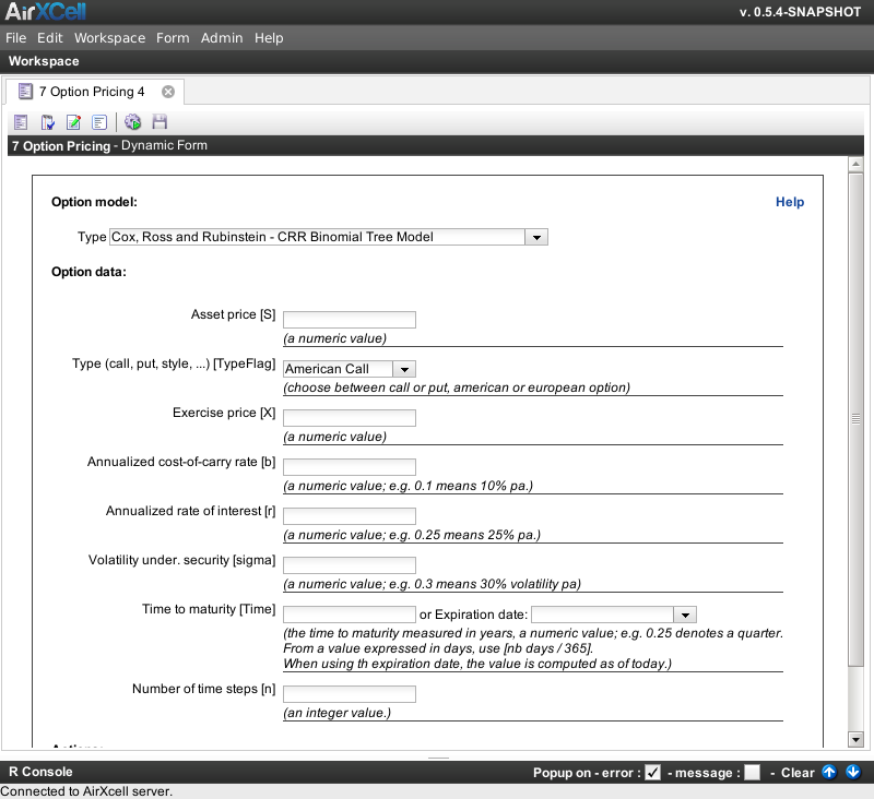
For instance, the Option pricing dynamic form using a binomial option model - here the Cox, Ross and Rubinstein, CRR Binomial Tree Model - looks as follows: Figure 16.2, “Binomial option pricing example”.

Figure 16.2. Binomial option pricing example

The supported variations of the binomial model are as follows:

16.3.2.1. Cox, Ross and Rubinstein - CRR Binomial Tree Model

Binomial models were first suggested by Cox, Ross and Rubinstein (1979) (CRR), and then became widely used because of its intuition and easy implementation. Binomial trees are constructed on a discrete-time lattice. With the time between two trading events shrinking to zero, the evolution of the price converges weakly to a lognormal diffusion.

Parameters are:

16.3.2.2. Jarrow and Rudd - JR Binomial Tree Model

There exist many extensions of the CRR model. Jarrow and Rudd (1983), JR, adjusted the CRR model to account for the local drift term. They constructed a binomial model where the first two moments of the discrete and continuous time return processes match. As a consequence a probability measure equal to one half results. Therefore the CRR and JR models are sometimes atrributed as equal jumps binomial trees and equal probabilities binomial trees.

Parameters are:

16.3.2.3. TIAN Binomial Tree Model

Tian (1993) suggested to match discrete and continuous local moments up to third order.

Parameters are:

16.3.3. European options

An option that can only be exercised at the end of its life, at its maturity. European options tend to sometimes trade at a discount to its comparable American option. This is because American options allow investors more opportunities to exercise the contract.

European options normally trade over the counter, while American options usually trade on standardized exchanges. A buyer of an European option that does not want to wait for maturity to exercise it can sell the option to close the position.

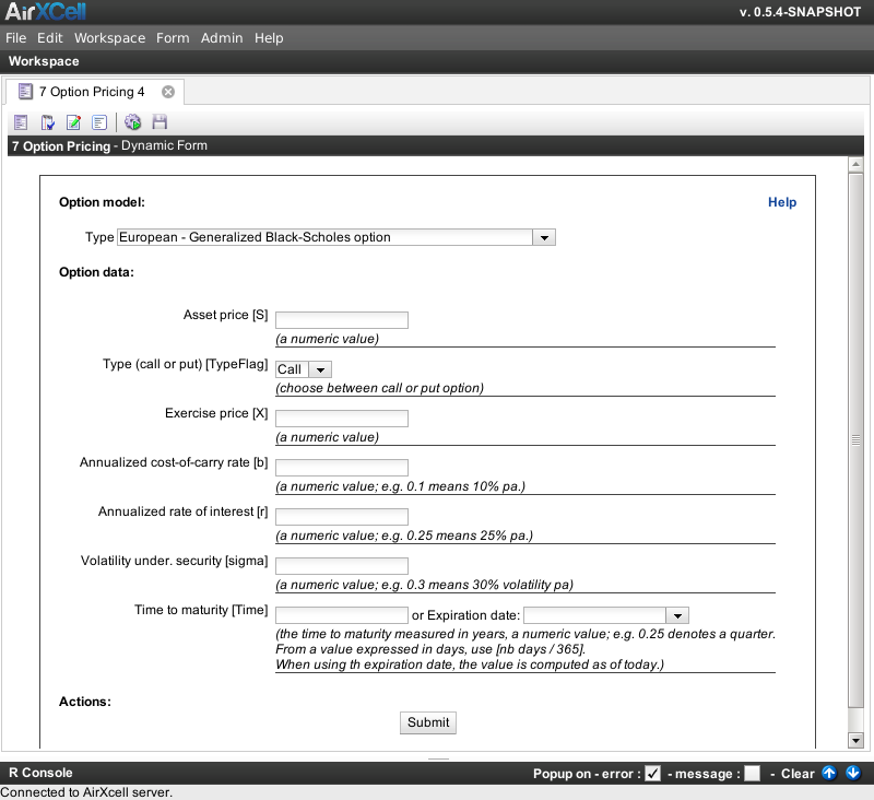
For instance, the Option pricing dynamic form using the generalized black-scholes model looks as follows: Figure 16.3, “European option pricing example”.

Figure 16.3. European option pricing example

16.3.3.1. Generalized Black Scholes Options

This consists in computing the option price following the Generalized Black scholes method.

Parameters are:

16.3.4. Asian options

For Asian options the payoff is determined by the average underlying price over some pre-set period of time. This is different from the case of the usual European option and American option, where the payoff of the option contract depends on the price of the underlying instrument at exercise; Asian options are thus one of the basic forms of exotic options.

One advantage of Asian options is that these reduce the risk of market manipulation of the underlying instrument at maturity. Another advantage of Asian options involves the relative cost of Asian options compared to European or American options. Because of the averaging feature, Asian options reduce the volatility inherent in the option; therefore, Asian options are typically cheaper than European or American options.

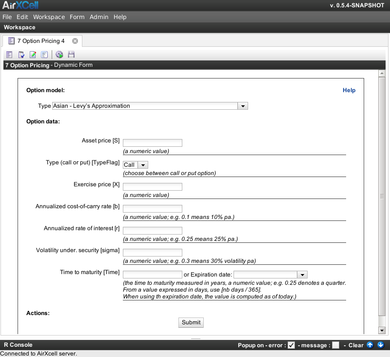
For instance, the Option pricing dynamic form using a asian option model - here the Levy's Approximation - looks as follows: Figure 16.4, “Asian option pricing example”.

Figure 16.4. Asian option pricing example

The supported models for asian options are as follows:

16.3.4.1. Geometric Average Rate Option

This uses the geometric average-rate option. The geometric average is the nth root of the product of the n sample points. Although Geometric Asian options are not commonly used in practice, they are often used as a good initial guess for the price of arithmetic Asian options

Parameters are:

16.3.4.2. Levy's Approximation

This uses the arithmetic average-rate option. The arithmetic average is the sum of the stock values divided by the number of sampling points. Here we ae using Levy's approximation.

Parameters are:

16.3.5. Barrier Options

A barrier option is an exotic derivative (here an option) on the underlying asset whose price breaching the pre-set barrier level either springs the option into existence or extinguishes an already existing option.

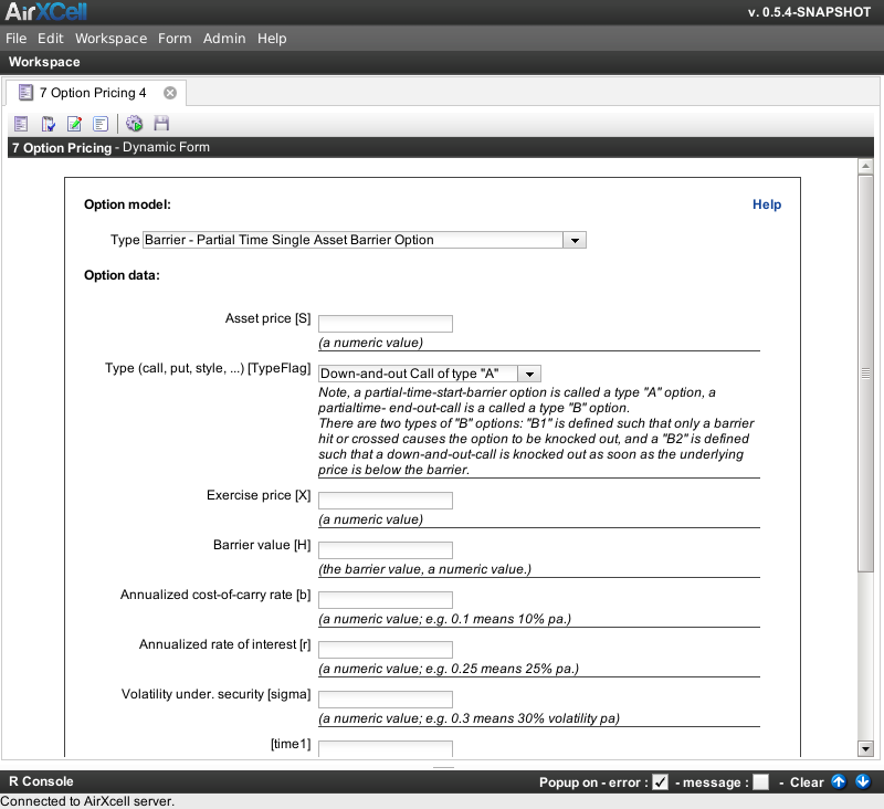
For instance, the Option pricing dynamic form using a barrier option model - here the Partial Time Single Asset Barrier Option - looks as follows: Figure 16.5, “Barrier option pricing example”.

Figure 16.5. Barrier option pricing example

Where the option springs into existence on the price of the underlying asset breaching a barrier, it may be known as an up and in, knock-in or down and in option.
Where the option is extinguished on the price of the underlying asset breaching a barrier, it may be known as an up and out, knock-out or down and out option.

Barrier options are always cheaper than a similar option without barrier. Thus, barrier options were created to provide the insurance value of an option without charging as much premium

The supported variations for barrier option models are as follows:

16.3.5.1. Standard Barrier Option

There are four types of single barrier options:

down-and-in call : comes into existence and knocked-in only if the asset price falls to the barrier level,
up-and-in call : comes into existence and knocked-in only if the asset price rises to the barrier level,
down-and-out call : comes into existence and knocked-out only if the asset price falls to the barrier level and
up-and-out call : comes into existence and knocked-out only if the asset price rises to the barrier level.

Parameters are:

16.3.5.2. Double Barrier Option

A double barrier option is either knocked in or knocked out if the asset price touches the lower or upper barrier during its lifetime. Once a barrier is crossed, the option comes into existence if it is a knock-in barrier or becomes worthless if it is a knocked out barrier.

Parameters are:

16.3.5.3. Partial Time Single Asset Barrier Option

For single asset partial-time barrier options, the monitoring period for a barrier crossing is confined to only a fraction of the option’s lifetime. There are two types of partial-time barrier options: partial-time-start and partial-time-end.

Partial-time-start barrier options : have the monitoring period start at time zero and end at an arbitrary date before expiration (called "A" type).
Partial-time-end barrier options : have the monitoring period start at an arbitrary date before expiration and end at expiration (called "B" type).

Partial-time-end barrier options are then broken down again into two categories: B1 and B2. Type B1 is defined such that only a barrier hit or crossed causes the option to be knocked out. There is no difference between up and down options. Type B2 options are defined such that a down-and-out call is knocked out as soon as the underlying price is below the barrier. Similarly, an up-and-out call is knocked out as soon as the underlying price is above the barrier.

Parameters are:

16.3.5.4. Two Asset Barrier Option

The underlying asset, Asset 1, determines how much the option is in or out-of-the-money. The other asset, Asset 2, is the trigger asset that is linked to barrier hits.

Parameters are:

16.3.5.5. Partial Time Two Asset Barrier Option

Partial-time two-asset barrier options are similar to standard two-asset barrier options, except that the barrier hits are monitored only for a fraction of the option’s lifetime. The option is knocked in or knocked out is Asset 2 hits the barrier during the monitoring period. The payoff depends on Asset 1 and the strike price.

Parameters are:

16.3.5.6. Lookback Barrier Option

A look-barrier option is the combination of a forward starting fixed strike Lookback option and a partial time barrier option. The option’s barrier monitoring period starts at time zero and ends at an arbitrary date before expiration. If the barrier is not triggered during this period, the fixed strike Lookback option will be kick off at the end of the barrier tenor.

Parameters are:

16.3.5.7. Discrete Barrier Option

TODO To Be Documented.

Parameters are:

16.3.5.8. Soft Barrier Option

A soft-barrier option is similar to a standard barrier option, except that the barrier is no longer a single level. Rather, it is a soft range between a lower level and an upper level. Soft-barrier options are knocked in or knocked out proportionally. Introduced by Hart and Ross (1994), the valuation formula can be used to price soft-down-and-in call and soft-up-and-in put options. The value of the related "out" option can be determined by subtracting the "in" option value from the value of a standard plain option.

Parameters are:

16.3.6. Binary Options

A binary option is a type of option where the payoff is either some fixed amount of some asset or nothing at all. The two main types of binary options are the cash-or-nothing binary option and the asset-or-nothing binary option. The cash-or-nothing binary option pays some fixed amount of cash if the option expires in-the-money while the asset-or-nothing pays the value of the underlying security. Thus, the options are binary in nature because there are only two possible outcomes. They are also called all-or-nothing options, digital options (more common in forex/interest rate markets), and Fixed Return Options (FROs) (on the American Stock Exchange). Binary options are usually European-style options.

For example, a purchase is made of a binary cash-or-nothing call option on XYZ Corp's stock struck at $100 with a binary payoff of $1000. Then, if at the future maturity date, the stock is trading at or above $100, $1000 is received. If its stock is trading below $100, nothing is received.

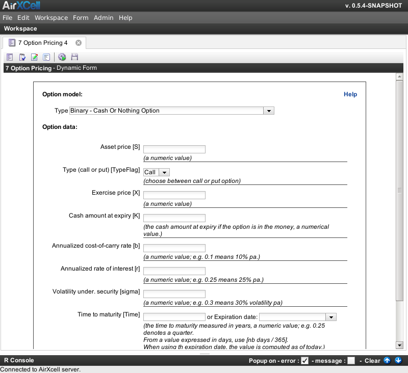
For instance, the Option pricing dynamic form using a binary option model - here the Cash Or Nothing Option Option - looks as follows: Figure 16.6, “Binary option pricing example”.

Figure 16.6. Binary option pricing example

The supported variations for binary option models are as follows:

16.3.6.1. Gap Option

The payoff on a gap option depends on the usual factors of a plain option, but is also affected by a "gap" amount of exercise prices, which may be positive or negative. Note, that a gap call (put) option is equivalent to being long (short) an asset-or-nothing call (put) and short (long) a cash-or-nothing call (put).

Parameters are:

16.3.6.2. Cash Or Nothing Option

For this option a predetermined amount is paid at expiration if the asset is above for a call or below for a put some strike level. The amount independent of the path taken. These options require no payment of an exercise price. The exercise price determines whether or not the option returns a payoff. The value of a cash-or-nothing call (put) option is the present value of the fixed cash payoff multiplied by the probability that the terminal price will be greater than (less than) the exercise price.

Parameters are:

16.3.6.3. Two Asset Cash Or Nothing Option

These options are building blocks for constructing more complex exotic options. There are four types of two-asset cash-or-nothing options, the first two situations are: A two-asset-cash-or-nothing call pays out a fixed cash amount if the price of the first asset is above (below) the strike price of the first asset and the price of the second asset is also above (below) the strike price of the second asset at expiration. The other two situations arise under the following conditions: A two-asset cash-or-nothing down-up pays out a fixed cash amount if the price of the first asset is is below (above) the strike price of the first asset and the price of the second asset is above (below) the strike price of the second asset at expiration.

Parameters are:

16.3.6.4. Asset Or Nothing Option

In this option a predetermined asset value is paid if the asset is, at expiration, above for a call or below for a put some strike level, independent of the path taken. For a call (put) the terminal price is greater than (less than) the exercise price, the call (put) expires worthless. The exercise price is never paid. Instead, the value of the asset relative to the exercise price determines whether or not the option returns a payoff. The value of an asset-or-nothing call (put) option is the present value of the asset multiplied by the probability that the terminal price will be greater than (less than) the exercise price.

Parameters are:

16.3.6.5. Super Share Option

These options represents a contingent claim on a fraction of the underlying portfolio. The contingency is that the value of the portfolio must lie between a lower and an upper bound at expiration. If the value lies within these boundaries, the supershare is worth a proportion of the assets underlying the portfolio, else the supershare expires worthless. A supershare has a payoff that is basically like a spread of two asset-or-nothing calls, in which the owner of a supershare purchases an asset-ornothing call with an strike price of the lower strike and sells an asset-or-nothing call with an strike price of the upper strike.

Parameters are:

16.3.7. Lookback Options

Lookback options are a type of exotic option with path dependency, among many other kind of options. The payoff depends on the optimal (maximum or minimum) underlying asset's price occurring over the life of the option. The option allows the holder to "look back" over time to determine the payoff. There exist two kinds of lookback options: with floating strike and with fixed strike.

The payoff from a pathdependent lookback call (put) depends on the exercise price being set to the minimum (maximum) asset price achieved during the life of the option. Thus, a lookback call (put) allows the purchaser to buy (sell) the asset at its minimum (maximum) price.

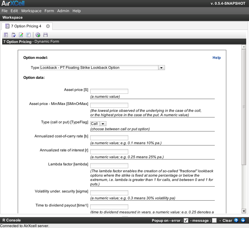
For instance, the Option pricing dynamic form using a lookback option model - here the Partial Ttime Floating Strike Lookback Option - looks as follows: Figure 16.7, “Lookback option pricing example”.

Figure 16.7. Lookback option pricing example

16.3.7.1. Floating Strike Lookback Option

The lookback call (put) option gives the holder the right to buy (sell) an asset at its lowest (highest) price observed during the life of the option. This observed price is applied as the strike price. The payout for a call option is essentially the asset price minus the minimum spot price observed during the life of the option. The payout for a put option is essentially the maximum spot price observed during the life of the option minus the asset price. Therefore, a floating strike lookback option is always in the money and should always be exercised.

Parameters are:

16.3.7.2. Fixed Strike Lookback Option

For a fixed strike lookback option, the strike price is known in advance. The call option payoff is given by the difference between the maximum observed price of the underlying asset during the life of the option and the fixed strike price. The put option payoff is given by the difference between the fixed strike price and the minimum observed price of the underlying asset during the life of the option. A fixed strike lookback call (put) option payoff is equal to that of a standard plain call (put) option when the final asset price is the maximum (minimum) observed value during the options life.

Parameters are:

16.3.7.3. PT Floating Strike Lookback Option

For a partial-time floating strike lookback option, the lookback period starts at time zero and ends at an arbitrary date before expiration. Except for the partial lookback period, the option is similar to a floating strike lookback option. The partial-time floating strike lookback option is cheaper than a similar standard floating strike lookback option.

Parameters are:

16.3.7.4. PT Fixed Strike Lookback Option

For a partial-time fixed strike lookback option, the lookback period starts at a predetermined date after the initialization date of the option. The partial-time fixed strike lookback call option payoff is given by the difference between the maximum observed price of the underlying asset during the lookback period and the fixed strike price. The partial-time fixed strike lookback put option payoff is given by the difference between the fixed strike price and the minimum observed price of the underlying asset during the lookback period. The partial-time fixed strike lookback option is cheaper than a similar standard fixed strike lookback option.

Parameters are:

16.3.8. Multiple Assets Options

Multiple asset options, as the name implies, are options whose payoff is based on two (or more) assets. The two assets are associated with one another through their correlation coefficient.

For instance, the Option pricing dynamic form using a multiple assets option model - here the Two Asset Correlation Option - looks as follows: Figure 16.8, “Multiple Assets option pricing example”.

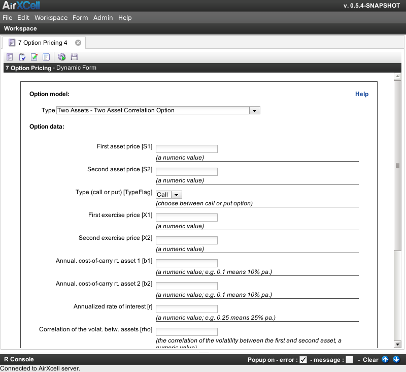
Figure 16.8. Multiple Assets option pricing example

16.3.8.1. Two Asset Correlation Option

A two asset correlation options have two underlying assets and two strike prices. A two asset correlation call option on two assets S1 and S2 with a strike prices X1 and X2 has a payoff of max(S2-X2,0) if S1 > X1 and 0 otherwise, and a put option has a payoff of max(X2-S2,0) if S1 < X1 and 0 otherwise.

Parameters are:

16.3.8.2. Exchange-One-Asset-For-Another Options:

Either European Exchange Option or American Exchange Option.

The exchange option gives the holder the right to exchange one asset for another. The payoff for this option is the difference between the prices of the two assets at expiration. The analytical calculation of European exchange option is based on a modified Black Scholes formula originally introduced by Margrabe (1978). A binomial lattice is used for the numerical calculation of an American or European style exchange option.

Parameters are:

16.3.8.3. Exchange Option on an Exchange Option

Exchange options on exchange options can be found embedded in many sequential exchange opportunities. As an example, a bond holder converting into a stock, later exchanging the shares received for stocks of an acquiring firm.

Parameters are:

16.3.8.4. Option on the Min/Max of 2 Risky Assets

TODO Document me

Parameters are:

16.3.9. Annexe : Calculation Model Parameters

All the parameters used by the various models above are presented and explained here:

16.3.9.1. [S] Asset price

[S] is the asset price, a numeric value.

16.3.9.2. [SMinOrMax] Lowest or Highest Aset price

[SMinOrMax] is the lowest price observed of the underlying in the case of a call, or the highest price in the case of a put. A numeric value.

16.3.9.3. [S1] Price of the first asset

[S1] is the price of the first asset, a numeric value.

16.3.9.4. [S2] Price of the second asset

[S2] is the price of the second asset, a numeric value.

16.3.9.5. [TypeFlag] Option type

Usually, [TypeFlag] is the type of the option, a character string either c for a call option or a p for a put option.

16.3.9.5.1. Binomial Models

In the case of the binomial models, the type can take the following values:

ce for European-Call
ca for American-Call
pe for European-Put
pa for American-Put

16.3.9.5.2. Double Barrier Option

In the special case of the Double Barrier Option, the type can take the following values:

co for up-and-out-down-and-out call
ci for up-and-in-down-and-in call
po for up-and-out-down-and-out put
pi for up-and-in-down-and-in put

16.3.9.5.3. Partial Time Single Asset Barrier Option

In the special case of the Partial Time Single Asset Barrier Option, the type can take the following values:

cdoA for down-and-out call of type "A"
cuoA for up-and-out call of type "A"
pdoA for down-and-out put of type "A"
puoA for up-and-out put of type "A"
coB1 for out-call of type "B1"
puoA for out-put of type "B1"
cdoB2 for down-and-out call of type "B2"
cuoB2 for up-and-out call of type "B2"

16.3.9.5.4. Soft and LookBack Barrier Option

In the special case of either of the Standard Barrier Option, the Soft Barrier Option and the Lookback Barrier Option, the type can take the following values:

cuo for up-and-out call
cdo for down-and-out call
cui for up-and-in call
cdi for down-and-in call
puo for up-and-out put
pdo for down-and-out put
pui for up-and-in put
pdi for down-and-in put

16.3.9.5.5. Two Asset Cash Or Nothing Option

In the special case of the Two Asset Cash Or Nothing Option, the type can take the following values:

c for a all option
o for a put option
ud for an up-down option
du for down-up option

16.3.9.5.6. Exchange-On-Exchange Option

In the special case of the Exchange-On-Exchange, the type can take the following values:

1 option to exchange Q * S2 for the option to exchange S2 for S1
2 option to exchange the option to exchange S2 for S1, in return for Q * S2
3 option to exchange Q * S2 for the option to exchange S1 for S2
4 option to exchange the option to exchange S1 for S2, in return for Q * S2

16.3.9.5.7. Exchange-On-Exchange Option

In the special case of the Exchange-On-Exchange, the type can take the following values:

cmin call on the minimum
cmax call on the maximum
pmin put on the minimum
pmax put on the maximum

16.3.9.6. [X] Exercise price

[C] is the exercise price - or the strike price, a numeric value.

16.3.9.7. [X1] First exercise price

[X1] is the first exercise price, a numeric value.

16.3.9.8. [X2] Second exercise price

[X2] is the second exercise price, a numeric value.

16.3.9.9. [XL] Lower boundary strike

[XL] is the lower limit of the exercise price, a numeric value.

16.3.9.10. [XH] Upper boundary strike

[XH] is the upper limit of the exercise price, a numeric value.

16.3.9.11. [b] Annualized cost-of-carry rate

[b] is the the annualized cost-of-carry rate, a numeric value; e.g. 0.1 means 10% pa.

16.3.9.12. [D] Dividend

[D] is a single dividend with time to dividend payout [time1].

16.3.9.13. [b1] Annualized cost-of-carry rate - First Asset

When working with a model based on two underlying assets, [b1] is the annualized cost-of-carry rate for the first asset, a numeric value; e.g. 0.1 means 10% pa.

16.3.9.14. [b2] Annualized cost-of-carry rate - Second Asset

When working with a model based on two underlying assets, [b2] is the annualized cost-of-carry rate for the second asset, a numeric value; e.g. 0.1 means 10% pa.

16.3.9.15. [H] Barrier Value

[H] is the barrier value, a numeric value.

16.3.9.16. [k] Prespecified Cash Rebate / Cash Amount at expiry

16.3.9.16.1. Standard Barrier Option

In the case of a Standard Barrier Option the [k] parameters denotes a prespecified cash rebate.

For an "In"-Barrier, [k] is the prespecified cash rebate which is paid out at option expiration if the option has not been knocked in during its lifetime.

For an "Out"-Barrier, [k] is the prespecified cash rebate which is paid out at option expiration if the option has not been knocked out before its lifetime, a numerical value.

16.3.9.16.2. Binary options

In the case of binary options - a Cash Or Nothing Option or a Two Assets Cash Or Nothing Option the [k] parameters denotes the cash amount at expiry.

In the case of a Cash Or Nothing Option, this is the cash amount at expiry if the option is in the money, a numerical value.

In the case of a Two Assets Cash Or Nothing Option this is the cash amount at expiry accordin to the following conditions:

for the cash-or-nothing call the cash amount at expiry if asset S1 is above the strike X1 and asset S2 is above strike X2 at expiration,
for the cash-or-nothing put the cash amount at expiry if asset S1 is below the strike X1 and asset S2 is below strike X2 at expiration,
for the cash-or-nothing up-down the cash amount at expiry if asset S1 is above the strike X1 and asset S2 is below strike X2 at expiration,
for the cash-or-nothing down-up the cash amount at expiry if asset S1 is below the strike X1 and asset S2 is above strike X2 at expiration.

16.3.9.17. [L] Lower limit of the barrier

[L] is the lower boundary to be touched, a numerical value.

16.3.9.18. [U] Upper limit of the barrier

[U] is the upper boundary to be touched, a numerical value.

16.3.9.19. [r] Annualized rate of interest

[r] is the annualized rate of interest, a numeric value; e.g. 0.25 means 25% pa.

16.3.9.20. [Q] Quantity both assets

[Q] is the quantity of both assets.

16.3.9.21. [Q1] Quantity first asset

[Q1] is the quantity of the first asset.

16.3.9.22. [Q2] Quantity first asset

[Q2] is the quantity of the second asset.

16.3.9.23. [rho] Correlation coefficient

[rho] is the correlation coefficient between the returns on the two assets.

16.3.9.24. [lamnda] Lambda Factor

The lambda factor enables the creation of so-called "fractional" lookback options where the strike is fixed at some percentage or below the extremum, i.e. lambda is greater than 1 for calls, and between 0 and 1 for puts.

16.3.9.25. [sigma] Annualized volatility

[sigma] is the annualized volatility of the underlying security, a numeric value; e.g. 0.3 means 30% volatility pa.

AirXCell provides a dynamic form to compuled annualized historical volatility from an underlying asset.

16.3.9.26. [sigma1] Annualized volatility first asset

[sigma1] is the annualized volatility of the first underlying security, a numeric value; e.g. 0.3 means 30% volatility p.a.

16.3.9.27. [sigma2] Annualized volatility second asset

[sigma2] is the annualized volatility of the second underlying security, a numeric value; e.g. 0.3 means 30% volatility p.a.

16.3.9.28. [delta1] numeric value for the curvature

Both [delta1] and [delta2] are numeric values which determine the curvature of the lower L and upper U bounds. The case of

delta1 = delta2 = 0 corresponds to two flat boundaries,
delta1 < 0 < delta2 correponds to a lower boundary exponentially growing as time elapses, while the upper boundary will be exponentially decaying,
delta1 > 0 > delta2 correponds to a convex downward lower boundary and a convex upward upper boundary

16.3.9.29. [delta2] numeric value for the curvature

See [delta1] numeric value for the curvature above.

16.3.9.30. [dt] Interval

[dt] is the time between moitoring instantes, i.e. the measured period, measured in years, a numeric value; e.g. 0.5 means 6 months.

16.3.9.31. [Time] Time to maturity

[Time] is the time to maturity measured in years, a numeric value; e.g. 0.5 means 6 months.

The time can either be input explicitely (for instance 0.6.) or computed using the date widget. When using the date widget, the time is computed as of today, i.e. the current date.

16.3.9.32. [time1] Time to Dividend Payout

[time1] measured the time to dividend payout in years, e.g. 0.25 denotes a quarter.

16.3.9.32.1. Partial Time Single/Two Asset(s) barrier option

In the case of a Partial Time Single Asset Barrier Option or a Partial Time Two Assets barrier Option, the options will have the location of the monitoring period starting at the options starting date and ending at an arbitrary time time1 before expiration time Time2. Partial-time-end-barrier options will have the location of the monitoring period starting at an arbitrary time time1 before expiration time Time2, and ending at expiration time.

16.3.9.32.2. Lookback Barrier Option

In the case of a Lookback Barrier Option, the lookbarrier option’s barrier monitoring period starts at the options starting date and ends at an arbitrary time time1 before expiration time Time2.

16.3.9.32.3. Partial Time Floating Strike Lookback Option

In the case of a Partial Time Floating Strike Lookback Option, thesee times are the time to the end of the lookback period time1, and the time to expiry Time2 where time1 < Time2.

16.3.9.32.4. Partial Time Fixed Strike Lookback Option

In the case of a Partial Time Fixed Strike Lookback Option, thesee times are the predetermined time time1 where the lookback period starts, and the time to expiry Time2.

16.3.9.33. [Time2] Time to maturity

[Time2] is the same as Section 16.3.9.31, “[Time] Time to maturity” for some other models.

16.3.9.33.1. Partial Time Single/Two Asset(s) barrier option

In the case of a Partial Time Single Asset Barrier Option or a Partial Time Two Assets barrier Option, the options will have the location of the monitoring period starting at the options starting date and ending at an arbitrary time time1 before expiration time Time2. Partial-time-end-barrier options will have the location of the monitoring period starting at an arbitrary time time1 before expiration time Time2, and ending at expiration time.

16.3.9.33.2. Lookback Barrier Option

16.3.9.33.3. Partial Time Floating Strike Lookback Option

In the case of a Partial Time Floating Strike Lookback Option, thesee times are the time to the end of the lookback period time1, and the time to expiry Time2 where time1 < Time2.

16.3.9.33.4. Partial Time Fixed Strike Lookback Option

In the case of a Partial Time Fixed Strike Lookback Option, thesee times are the predetermined time time1 where the lookback period starts, and the time to expiry Time2.

16.3.9.34. [n] Number of Time Steps

[n] is the numbre of time steps, an integer value.

16.4. Results

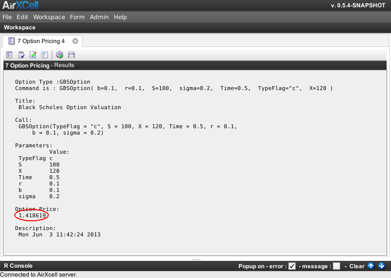
As with other dynamic forms, the resulting computed price is displayed in the result panel.

For instance the result of a Generalized Black Scholes Option as computed with AirXCell and displayed in the result panel is shown on figure Figure 16.9, “Generalized Black Scholes Option Price Result”.

Figure 16.9. Generalized Black Scholes Option Price Result

Prev		Next
Chapter 15. Form : 6. Portfolio Optimization	Home	Chapter 17. Portfolio Optimization theory