Copyright © 2011-2014 airxc.com, airxcell.com
Table of Contents
This chapter presents a quick overview of the underlying theoretical math concepts used by the portfolio optimization procedures implemented in the Portfolio (15) dynamic form. Both methodologies on which are built the optimization algorithms are presented, namely the Markowitz Portfolio Theory and the Mean-CVaR Portfolio Theory.
Most of the concepts presented here are compiled from several reference books on this specific field such as [10] and [11]. Moreover, the following documents available online provide interesting additional insights: [7], [10] and [3].
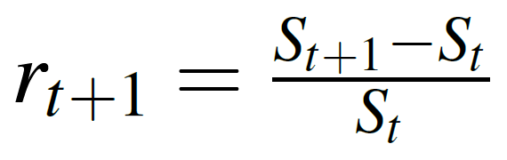
In financial engineering, we often work with asset returns instead of asset prices. Given a financial instrument's price St where t denotes the period, the discrete return rt + 1 between t and t + 1 is defined as:
 |
The concepts presented in this section are largely inspired from [6], [7] and [10].
In this section we define the original mean-variance portfolio optimization problem and several related problems. The problem of minimizing the covariance risk for a given target return with optional box and group constraints is a quadratic programming problem with linear constraints. We call this problem minimum risk mean-variance portfolio.
The opposite case, fixing the risk and maximizing the return, has a linear objective function with quadratic constraints. We call this programming problem the maximum return mean- variance portfolio problem. This problem is much more complex than the previous one.
If we have even more complex constraints, i.e. nonlinear constraints, we need a new class of solvers. This is called non-linear constrained portfolio problem. This allows us to handle the case of linear and quadratic objective functions with non-linear constraints. In all three cases we speak of Markowitz' portfolio optimization problem, although they require different classes of solvers with increasing complexity.
Following Markowitz we define the problem of portfolio selection as follows:
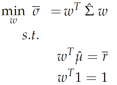 |
The formula expresses that we minimize the variance - covariance risk σ̄ , where the matrix Σ̂ is an estimate of the covariance of the assets. The vector ω denotes the individual investments subject to the condition ωT 1 = 1 that the available capital is fully invested. The expected or target return r̄ is expressed by the condition ωT μ̂ = r̄ , where the p-dimensional vector μ̂ estimates the expected mean of the assets.
Markowitz' portfolio modell has a unique solution:
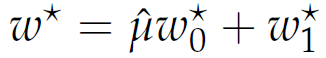 |
where
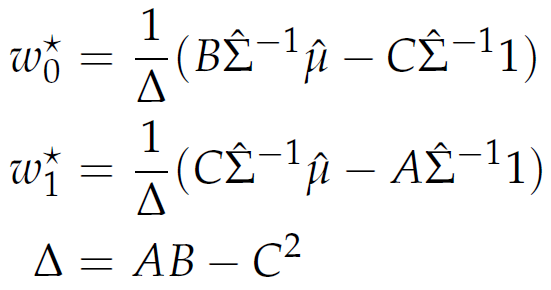 |
with
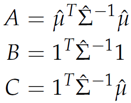 |
The corresponding standard deviation σ̄ for the optimal portfolio with weights ω* is
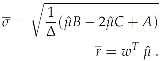 |
The locus of this set in the { σ̄ , r̄ }-space are hyperbolas. The set inside the hyperbola is the feasible set of mean/standard deviation portfolios, and the borders are the efficient frontier (upper border), and the minimum variance locus (lower border). Here, r* is the return of the minimum variance portfolio.
The point with the smallest risk on the efficient frontier is called the global minimum variance portfolio, MVP. The MVP represents just the minimum risk point on the efficient frontier.The set of weight is:
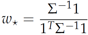 |
In contrast to minimum risk portfolios, where we minimize the risk for a given target return, maximum return portfolios work the opposite way: Maximize the return for a given target risk.
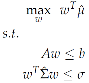 |
Note that now we are concerned with a linear programming problem and quadratic constraints. This can be solved in the Portfolio optimization (15) dynamic form using the available linear solver (15.4.5).
The concepts presented in this section are largely inspired from [2], [3] and [10].
In this chapter we formulate and solve the mean-CVaR portfolio model, where covariance risk is now replaced by the conditional Value at Risk as the risk measure. In contrast to the mean-variance portfolio optimization problem, we no longer assume the restriction consisting in the set of assets to have a multivariate elliptically contoured distribution.
We consider a portfolio of assets with random returns. We denote the portfolio vector of weights with ω and the random events by the vector r. Let f ( ω , r) denote the loss function when we choose the portfolio W from a set X of feasible portfolios and let r be the realization of the random events.We assume that the random vector r has a probability density function denoted by p(r). For a fixed decision vector ω , we compute the cumulative distribution function of the loss associated with that vector ω.
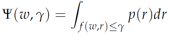 |
Then, for a given confidence level α, the VaRα associated with portfolio W is given as
 |
Similarly, we define the CVaRα associated with portfolio W
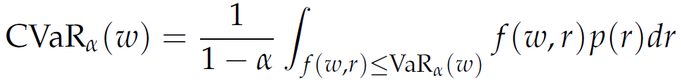 |
We then define the problem of mean-CVaR portfolio selection as follows:
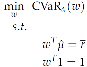 |
In general, minimizing CVaRα and VaRα are not equivalent. Since the definition of CVaRα involves the VaRα function explicitly, it is difficult to optimize or work with this function. Instead, we consider the following simpler auxiliary function:
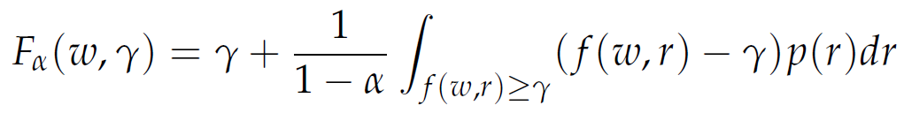 |
Alternatively, we can write Fα(ω, γ) as follows:
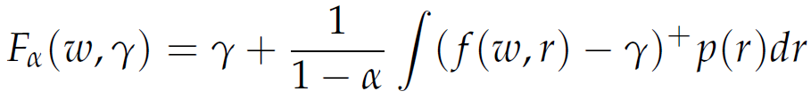 |
where z+ = max(z, 0). This final function of γ has the following important properties that make it useful for the computation of CVaRα and VaRα:
- Fα(ω, γ) is a convex function of γ,
- VaRα(ω) is a minimizer of Fα(ω, γ),
- the minimum value of the function Fα(ω, γ)) is CVaRα(ω).
As a consequence, we deduce that CVaRα can be optimized via optimization of the function Fα(ω, γ) with respect to the weights w and VaR g. If the loss function f (ω, r) is a convex function of the portfolio variables w, then Fα(ω, γ) is also a convex function of ω. In this case, provided the feasible portfolio set ω is also convex, the optimization problems are smooth convex optimization problems that can be solved using well-known optimization techniques for such problems.
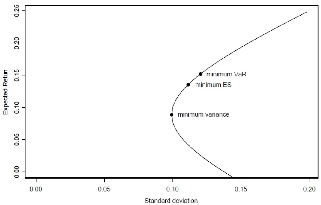
Figure Figure 17.1, “Efficient mean-variance frontier [8]” shows the Efficient mean-variance frontier with the global minimum variance portfolio, the global minimum Value at Risk (5%) portfolio and the global minimum Conditional Value at Risk (5%) portfolio. The efficient frontiers under the various measures, are the subset of boundaries above the corresponding minimum global risk portfolios. We see that under 5% VaR and 5% CVaR the set of efficient portfolios is reduced with respect to the variance.
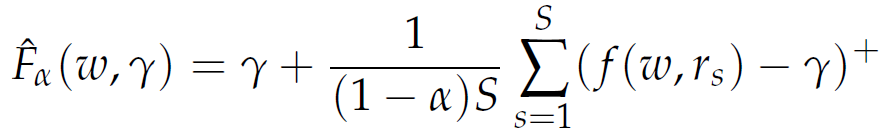
Often it is not possible or desirable to compute/determine the joint density function p(r) of the random events in our formulation. Instead, we may have a number of scenarios, say rs for s = 1, ... , S, which may represent some historical values of the returns. In this case, we obtain the following approximation to the function Fα(ω, γ) by using the empirical distribution of the random returns based on the available scenarios:
 |
Now, the problem minω∈W CVaRα(ω) can be approximated by
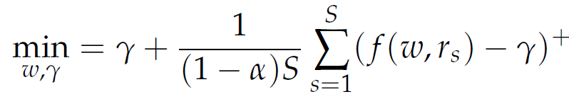 |
To solve this optimization problem, we introduce artificial variables zs to replace (f(ω, rs) - γ)+. This is achieved by imposing the constraints zs ≥ f(ω, rs) - γ and zs ≥ 0.
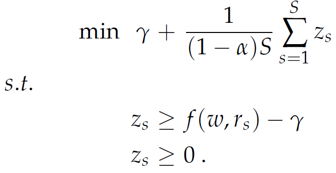 |
Note that the constraints zs ≥ f(ω, rs) - γ and zs ≥ 0 alone cannot ensure that zs = (f(ω, rs) - γ)+, since zs can be larger than both right-hand term and still be feasible. However, since we are minimizing the objective function, which involves a positive multiple of zs, it will never be optimal to assign zs a value larger than the maximum of the two quantities f(ω, rs) - γ and 0, and therefore, in an optimal solution zs will be precisely (f(ω, rs) - γ)+, thus justifying our substitution.
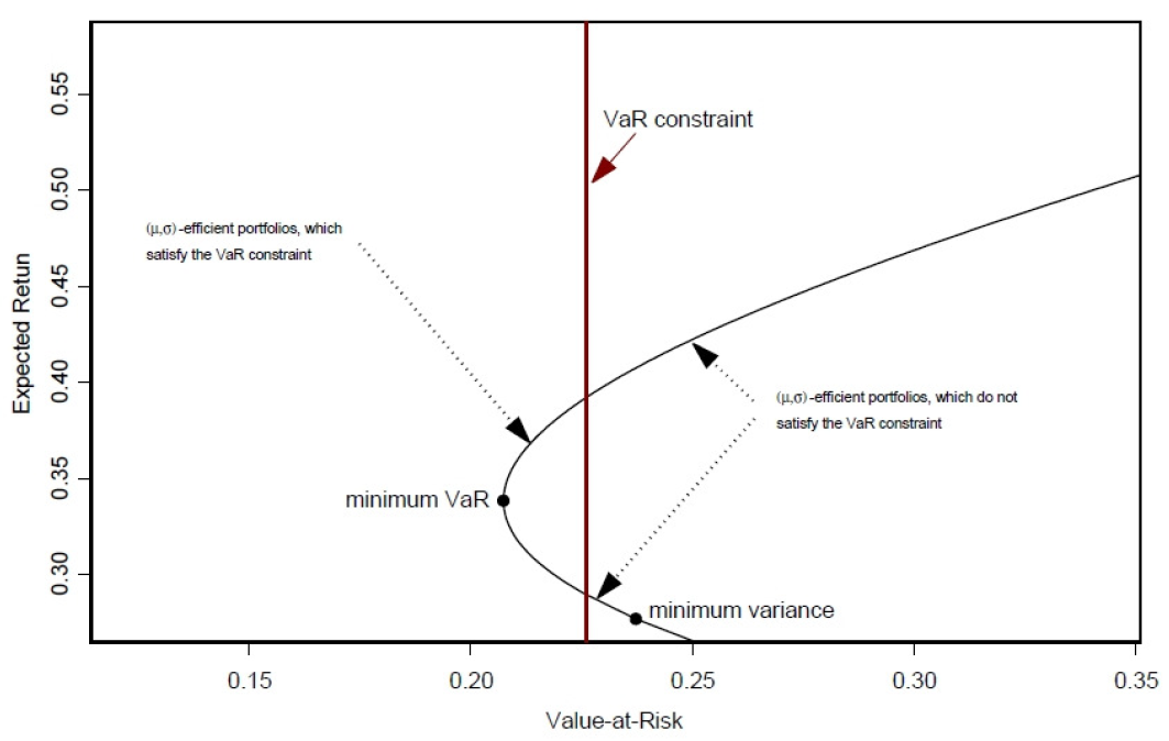
Figure Figure 17.2, “Mean-VaR(5%)-boundary [8]” shows the Mean-VaR(5%)-boundary with the global minimum variance portfolio. Portfolios on the mean-VaR(5%)-boundary between the global minimum VaR( 5%) portfolio and the global minimum variance portfolio, are mean-variance efficient. The VaR constraint (vertical line) could force mean-variance investors with high variance to reduce the variance, and mean-variance investors with low variance to increase the variance, in order to be on the left side of the VaR constraint.
In the case that f(ω, rs) - γ is linear in ω , all the expressions zs ≥ f(ω, rs) - γ represent linear constraints and therefore the optimization problem becomes a linear programming problem that can be solved using the simplex method or alternative linear programming algorithms.