Copyright © 2011-2014 airxc.com, airxcell.com
Table of Contents
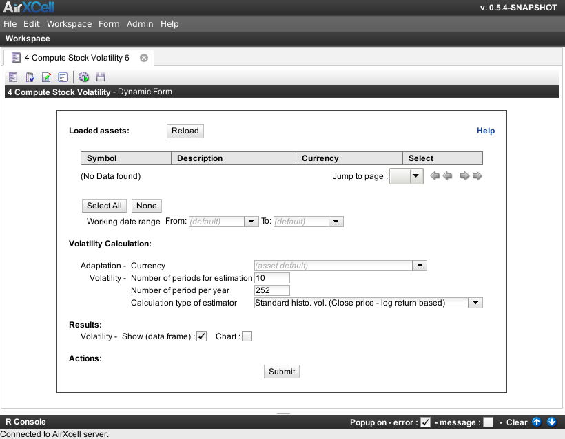
This dynamic form is about historical stock volatility calculation. It provides the user with a mean to compute the volatility of an underlying asset.
TODO
Quoting wikipedia : In finance, volatility is a measure for variation of price of a financial instrument over time. Historic volatility is derived from time series of past market prices. An implied volatility is derived from the market price of a market traded derivative (in particular an option).
Volatility as described here refers to the actual current volatility of a financial instrument for a specified period (for example 30 days or 90 days). It is the volatility of a financial instrument based on historical prices over the specified period with the last observation the most recent price.
For instance, the figure Figure 13.1, “4. Compute stock volatility” shows a"4. Compute stock volatility" form :
The annualized volatility σ is the standard deviation of the instrument's yearly logarithmic returns.
Stock prices are usually observed at fixed intervals of time (daily, weekly or monthly) and we then have a time series of data. The log relative returns are mathematically defined by the equation:
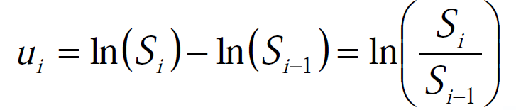 |
where : i S is the stock price at the end of the i -th interval and ln( ) is the natural logarithmic function.
- Si is the i-th interval and
- ln() is the natural logarithmic function
Volatility is defined as the variation or dispersion or deviation of an asset's returns from their mean. Large values of volatility mean that returns fluctuate in a wide range (large risk). The most common measure of dispersion is the standard deviation of a random variable.
In their paper in 1973, Black & Scholes mentioned the parameter σ2 which they said was the ""variance rate of the return" on the stock prices. Black & Scholes took this as a known parameter that is constant through the life of the option.
In a paper prior to their seminal one, Black & Scholes gave more insight into the variance rate of return. There they stated that they estimated the instantaneous variance from the historical series of daily stock prices. They thus defined volatility as the amount of variability in the returns of the underlying asset. Black & Scholes determined what is today known as the historical volatility and used that as a proxy for the expected volatility in the future.
To estimate the volatility of a stock price empirically, the stock price is usually observed at fixed intervals of time. These intervals can be days, weeks or months. It is well admitted that days when the exchange is closed should be ignored.
The historical volatility is the volatility of a series of stock prices where we look back over the historical price path of the particular stock. We previously mentioned that the most common measure of dispersion is the standard deviation. The daily historical volatility estimate is thus given by:
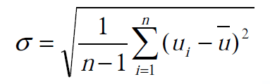 |
where μ̂ is the mean defined by:
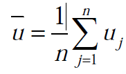 |
The given volatility is the estimated volatility per interval also called sometimes the daily volatility.
To be able to compare volatilities for different interval lengths we express usually the volatility in annual terms. To do this we scale this estimate with an annualization factor (normalizing constant) h which is the number of intervals per annum such that:
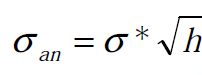 |
If daily data is used the interval is one trading day and we use h = 252, if the interval is a week, h = 52 and h = 12 for monthly data.
A simple option pricing model (like the Black & Scholes model) will give a theoretical price for an option as a function of the implicit parameters — constant volatility being one. However, if the option is traded, the market price might not be the same as the model price.
In that case one might ask, which volatility estimate does one have to use in the model so that the model price and the market price are the same? This is the implied volatility.
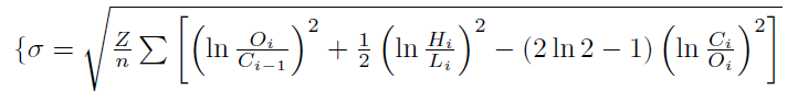
The Garman and Klass estimator for estimating historical volatility assumes Brownian motion with zero drift and no opening jumps (i.e. the opening = close of the previous period). This estimator is 7.4 times more efficient than the close-to-close estimator.
 |
The Parkinson formula for estimating the historical volatility of an underlying based on high and low prices during the day.
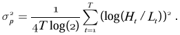 |
The Roger and Satchell historical volatility estimator allows for non-zero drift, but assumed no opening jump.
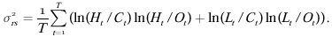 |
This estimator is a modified version of the Garman and Klass estimator that allows for opening gaps.
Yang and Zhang derived an extension to the Garman Glass historical volatility estimator that allows for opening jumps. It assumes Brownian motion with zero drift. This is currently the preferred version of open-high-low-close volatility estimator for zero drift and has an efficiency of 8 times the classic close-to-close estimator. Note that when the drift is nonzero, but instead relative large to the volatility, this estimator will tend to overestimate the volatility.
 |
The Yang and Zhang historical volatility estimator has minimum estimation error, and is independent of drift and opening gaps. It can be interpreted as a weighted average of the Rogers and Satchell estimator, the close-open volatility, and the open-close volatility.