Copyright © 2011-2014 airxc.com, airxcell.com
Table of Contents
Technical and quantitative analysts have applied statistical principles to the financial market since its inception. Some attempts have been very successful while some have been anything but. The key is to find a way to identify price trends without the fallibility and bias of the human mind. One approach that can be successful for investors and is available in most charting tools is Simple linear regression.
Linear regression analyzes two separate variables in order to define a single relationship. In our case, we will use the two variables available on an asset or FOREX quotes timeseries, hence the price and time variables.
Describing the detailed statistical and mathematical approach behind computing a Simple linear regression is beyond the scope of this document. But we will walk through the various steps required within AirXCell to compute such a simple linear regression on asset or FOREX quotes.
We will cover here two different methods for computing and charting a Simple Linear Regression on asset or FOREX quotes:
The first way consists in doing it manually using the
fRegressionR package and an R console or the R Code Editor.The second way consists in using the 5 analyze assets form.
One should thoroughly follow How-to How To : Load Asset or FOREX quotes within AirXCell (3) before running the next sections.
The remainder of this chapter assumes the user has execute that previous How-To and continues here right at its end.
The procedure is pretty straightforward with the help of the fRegression package and its
regFit method.
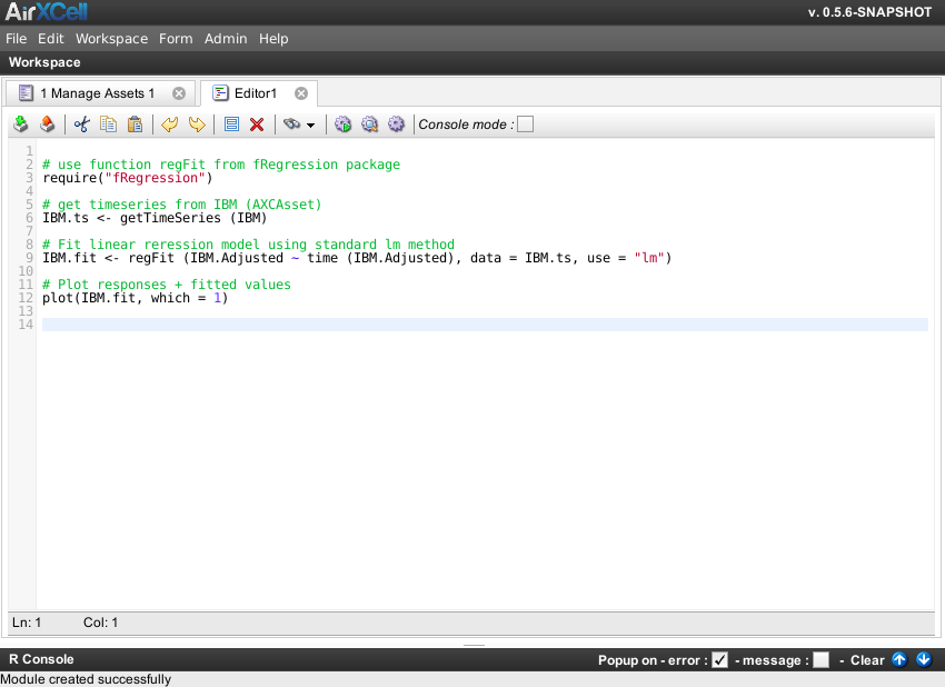
The R code we will be using is as follows:
# use function regFit from fRegression package
require("fRegression")

# get timeseries from IBM (AXCAsset)
IBM.ts <- getTimeSeries (IBM)

# Fit linear reression model using standard lm method
IBM.fit <- regFit (IBM.Adjusted ~ time (IBM.Adjusted), data = IBM.ts, use = "lm")

# Plot responses + fitted values
plot(IBM.fit, which = 1)

# Plot residuals
plot(IBM.fit, which = 2)
It's quite sefl-explanatory. Let's just underline the function we are using :
IBM.Adjusted ~ time (IBM.Adjusted) where IBM.Adjusted is the title of the column
of the timeseries that contains adjusted prices.
The formula hence means that we eant to perform a simple linear regression of the asset adjusted quotes against the time of the quotes.
Once the IBM Asset quotes are loaded, we should open an R Code Editor and type in the code above.
The result is shown on Figure 5.1, “Regression calculation code in editor”:
One can execute the code using either Ctrl + A typed in the editor or the "Run All" button
on the toolbar.
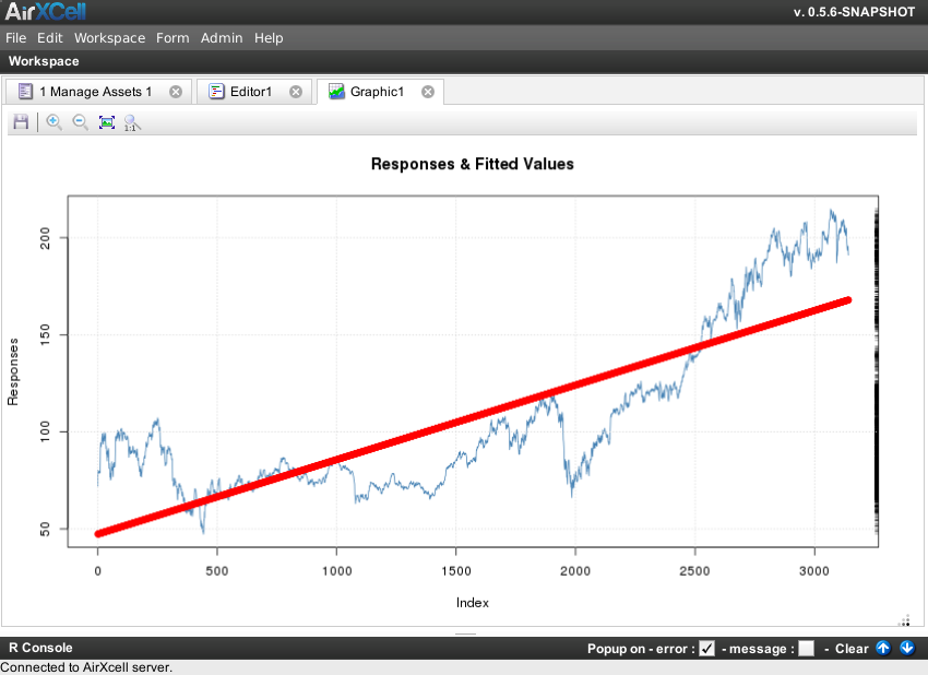
The result from the execution is shown on Figure 5.2, “Responses + Fitted values”:
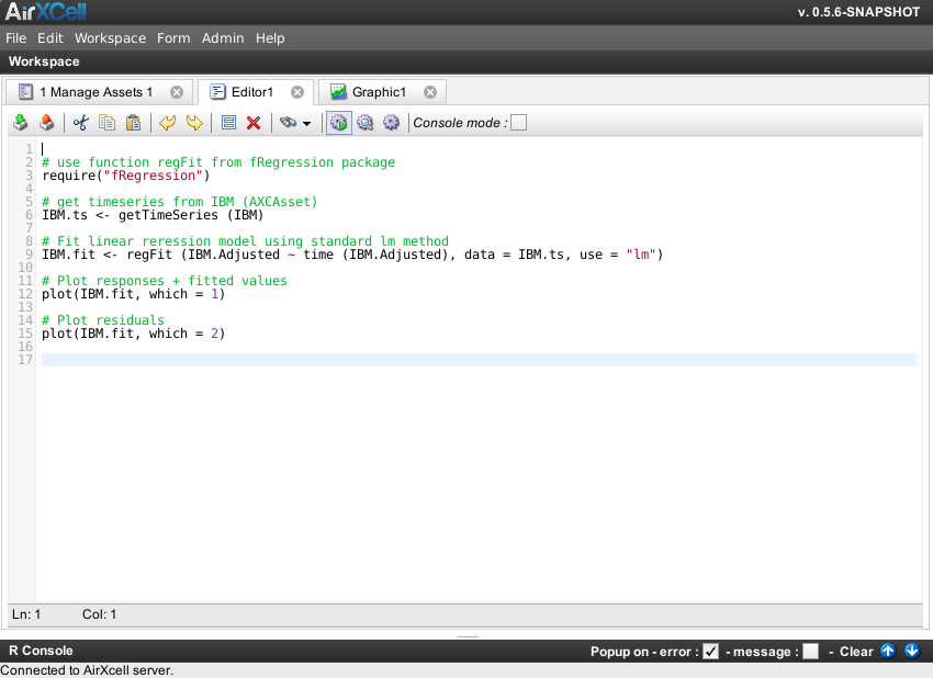
Let's now change the code in the editor a little bit to chart the residuals in addition to the fitted values.
The R code we will be using for this is :
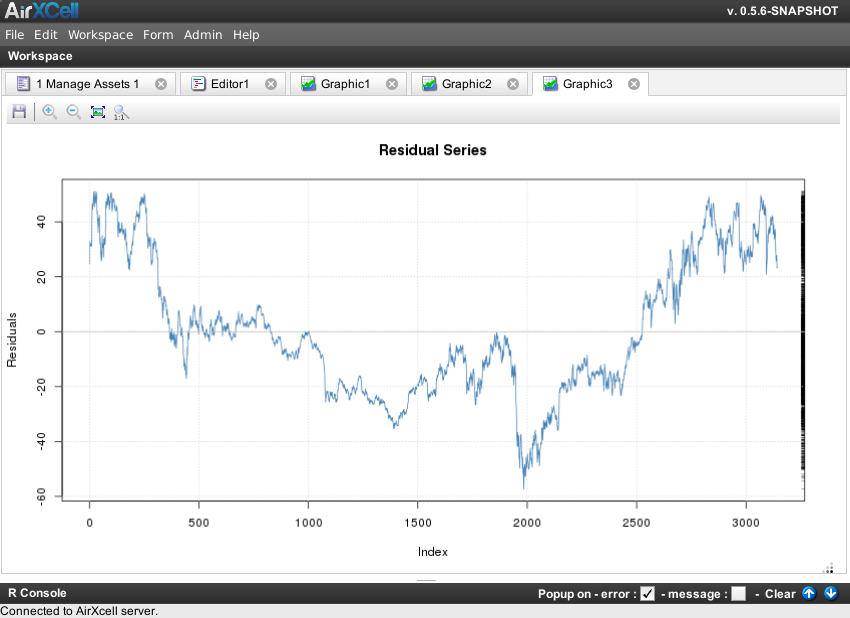
# Plot residuals
plot(IBM.fit, which = 2)
The new code is shown on Figure 5.3, “Regression calculation code in editor (2)”:
The result from the execution is shown on Figure 5.4, “Residuals”:
With the manual way, any kind of regression can be computed within AirXCell, the user just needs the data loaded within AirXCell as timeseries and define the right formula.
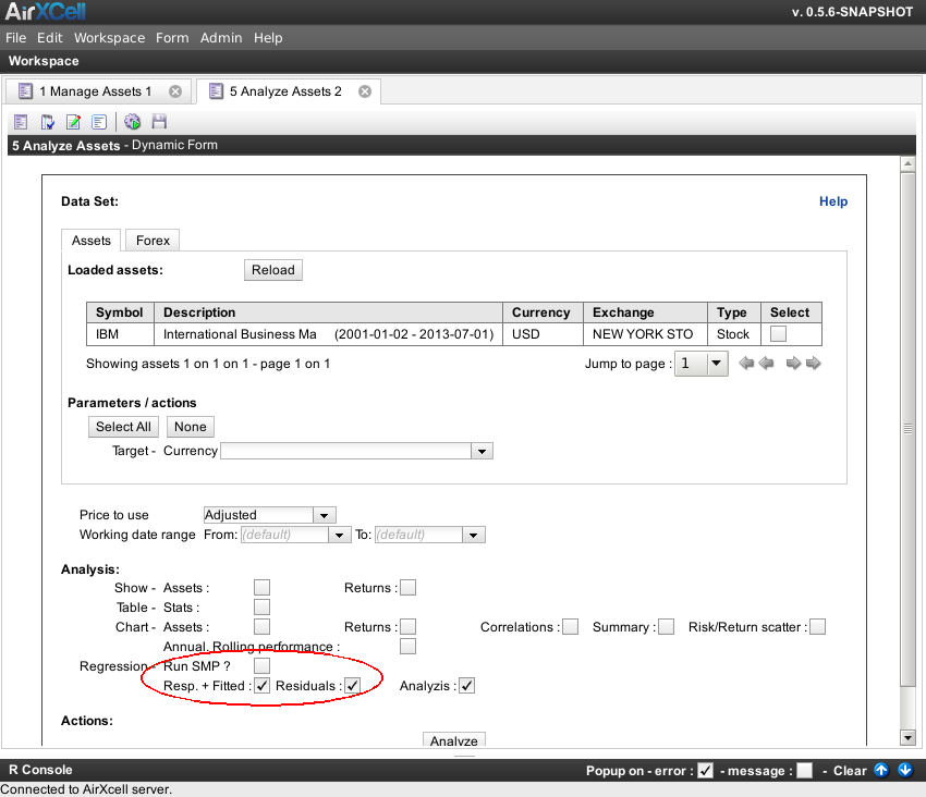
As stated previously, a simple linear regression on asset quotes can be computed automatically with the help of the 5 analyze assets form.
One simply needs to open such a form, select the desired asset and run SMP as shown on Figure 5.5, “Automatically running SMP”: