AirXCell provides various "forms" aimed at simplifying the loading, manipulation and visualization of Asset and FOREX quote timeseries. The 1. Manage Asset form provides the user with a mean to load timeseries, manipulate them, visualize them, etc.

In addition, an asset quote timeseries is always loaded in the asset trading currency. AirXCell provides a way to display any asset quote timeseries in any arbitrary currency. It takes care automatically of the loading of the required FOREX timeseries for the asset timeseries period and applies it to the asset quotes.

While this can easily be performed manually by the user in the R console or using an R Code Editor, the 1. Manage Asset form provides a way to do it only in a few clicks

One should thoroughly follow How-to How To : Load Asset or FOREX quotes within AirXCell (3) before running the next sections.

The remainder of this chapter assumes the user has execute that previous How-To and continues here right at its end.

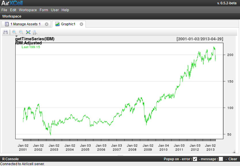
Before applying any FOREX to our 'IBM' quote timeseries by selecting an arbitrary target currency, let's just chart the IBM quote timeseries using the native currency. The native currency here is displayed on the list of results beneath the name of the asset. In out case the native currency is 'USD'.

One can display a chart of the IBM quote timeseries using the "chart" button as shown on Figure 4.1, “Chart IBM in native currency”:

The system opens a new module of type "Graphic" and adds it in the user workspace as shown on Figure 4.2, “IBM in native currency”:

We can now close this module and move to the next step which is chosing a different currency.

Back to the 1. Manage Asset form, the user can choose a different currency and use it to display the asset in a different, arbitrary currency by fully appliying the FOREX quote timeseries to the Asset quote timeseries.

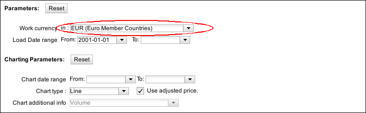
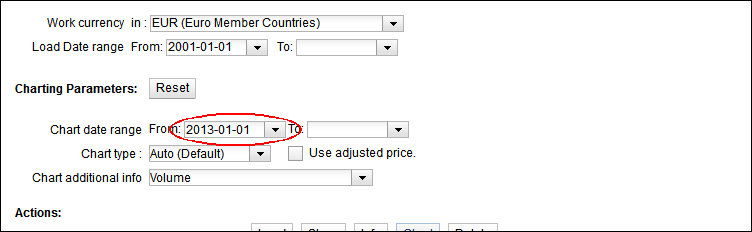
First, we need to set the "Work currency" to 'EUR' as shown on Figure 4.3, “Chart IBM in native currency (USD)”:

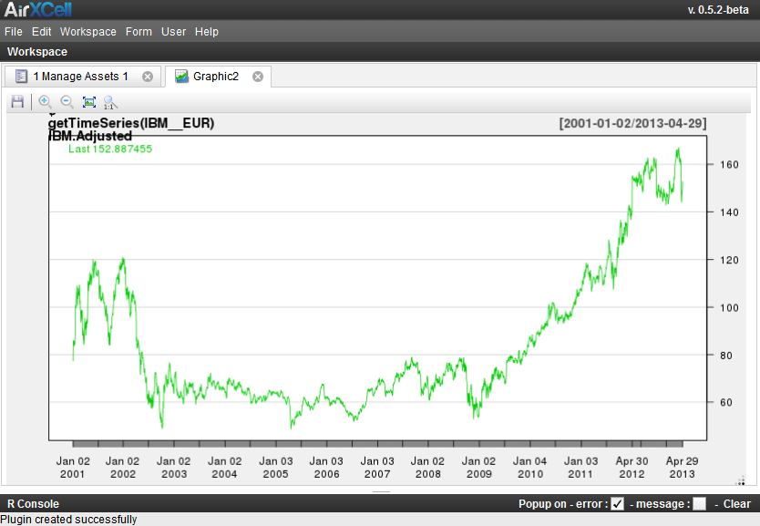
We can now press the 'Chart' button again to display the 'IBM' asset quote timeseries in 'EUR' as shown on Figure 4.4, “IBM in euros (EUR)”:

We will now display the IBM quote timeseries in euros for the last year using candlesticks. It doesn't make much sense using candlestick to display much more than one years since the chart quickly becomes unreadable.

First we unchedk the "Use Adjusted" box and select back the value "auto" as Chart Type.

Second we select "2013-01-01" as start date for the chart as shown on figure Figure 4.5, “Using a chart start date”:

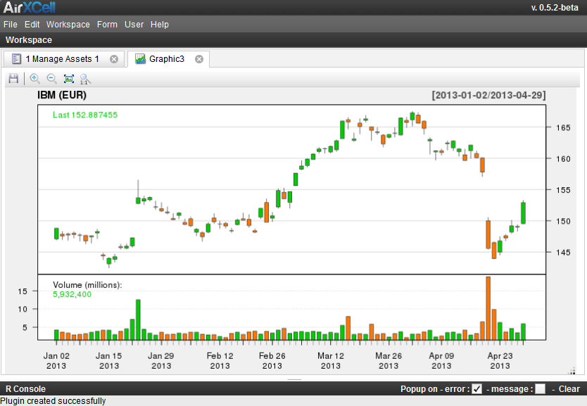
We can now press the 'Chart' button again to display the 'IBM' asset quote timeseries in 'EUR' for last year using candlesticks as shown on Figure 4.6, “IBM in euros (EUR) with candlesticks”:

We can now keep this graphic module open but switch back to the 1. Manage Asset form to display the timeseries in a Data Frame Editor module.

We will now use a Data Frame Editor module to display the IBM quote timeseries and be able to edit it should we want to.

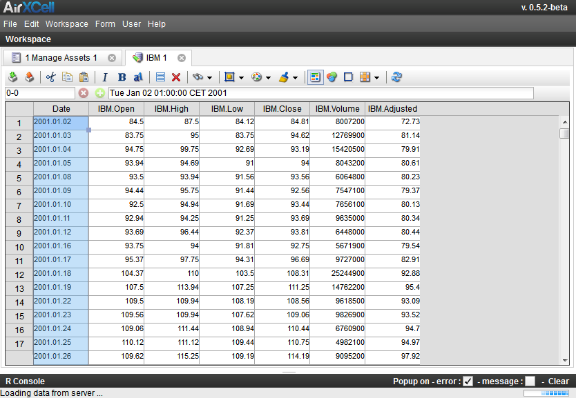
Back to the 1. Manage Asset form, this is simply performed by clicking the "Show" button on the bottom of the form as shown on Figure 4.7, “Show the timeseries in a data frame module”:

The system opens a new module which showns the timeseries as shown on Figure 4.8, “The raw presentation of the timeseries”:

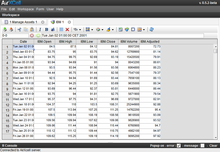
As of current version of AirXCell, the format of the first column - the date - is not properly recognized by the User Interface module. We should change the presentation format of this data to get a better representation of the data frame.

First, let's start by selecting the first column by clicking on the header and trhen pressing the "Choose data format" button as shown on Figure 4.9, “Chosing the data format”:

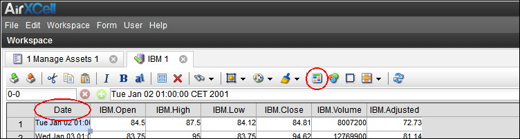
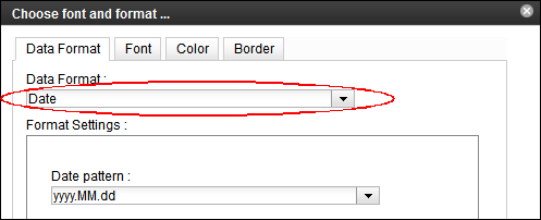
We are then presented to the Data Frame Format screen where the "Data Format" tab has been preselected. At this point we're left with chosing the right format - 'date' - as shown on Figure 4.10, “Switch to Date format”:

The result is a much better presentation as shown on Figure 4.11, “The timeseries with a better presentation”: